The normal model with pymc

Normal Model for fixed $\sigma$
Example of the normal model for fixed $\sigma$
Sampling by code
Sampling with pymc
- Results
Letting $\sigma$ be a stochastic

%matplotlib inline
import numpy as np
import matplotlib.pylab as plt 
import seaborn as sns

from scipy.stats import norm

A random variable $Y$ is normally distributed with mean $\mu$ and variance $\sigma^2$. Thus its density is given by :

$p(y \vert \mu, \sigma^2) = \frac{1}{ \sqrt{ 2 \pi \sigma^2}} e^{-( \frac{y-\mu}{2 \sigma})^2}$

Suppose our model is ${y_1, \ldots, y_n \vert \mu, \sigma^2 } \sim N(\mu, \sigma^2)$ then the likelihood is

$p(y_1, \ldots, y_n \vert \mu, \sigma^2) = \prod_{i=1}^{n} p(y_i \vert \mu, \sigma^2)=\prod_{i=1}^{n} \frac{1}{ \sqrt{ 2 \pi \sigma^2}} e^{-( \frac{(y_i-\mu)^2}{2\sigma^2})} = \frac{1}{ \sqrt{ 2 \pi \sigma^2}} \exp \left\{ - \frac{1}{2} \sum_i \frac{(y_i-\mu)^2}{\sigma^2} \right\}$

We can now write the posterior for this model thus:

$p( \mu, \sigma^2 \vert y_1, \ldots, y_n, \sigma^2) \propto \frac{1}{ \sqrt{ 2 \pi \sigma^2}} e^{ - \frac{1}{2\sigma^2} \sum (y_i - \mu)^2 } \, p(\mu, \sigma^2)$

Lets see the posterior of $\mu$ assuming we know $\sigma^2$.

Normal Model for fixed $\sigma$

Now we wish to condition on a known $\sigma^2$. The prior probability distribution for it can then be written as:

$p(\sigma^2) = \delta(\sigma^2 -\sigma_0^2)$

(which does integrate to 1).

Now, keeping in mind that $p(\mu, \sigma^2) = p(\mu \vert \sigma^2) p(\sigma^2)$ and carrying out the integral over $\sigma^2$ which because of the delta distribution means that we must just substitute $\sigma_0^2$ in, we get:

$p( \mu \vert y_1, \ldots, y_n, \sigma^2 = \sigma_0^2) \propto p(\mu \vert \sigma^2=\sigma_0^2) \,e^{ - \frac{1}{2\sigma_0^2} \sum (y_i - \mu)^2 }$

where I have dropped the $\frac{1}{\sqrt{2\pi\sigma_0^2}}$ factor as there is no stochasticity in it (its fixed).

Say we have the prior

$p(\mu \vert \sigma^2) = \exp \left\{ -\frac{1}{2 \tau^2} (\hat{\mu}-\mu)^2 \right\}$

Example of the normal model for fixed $\sigma$

We have data on the wing length in millimeters of a nine members of a particular species of moth. We wish to make inferences from those measurements on the population mean $\mu$. Other studies show the wing length to be around 19 mm. We also know that the length must be positive. We can choose a prior that is normal and most of the density is above zero ($\mu=19.5,\tau=10$). This is only a marginally informative prior.

Many bayesians would prefer you choose relatively uninformative (and thus weakly regularizing) priors. This keeps the posterior in-line (it really does help a sampler remain in important regions), but does not add too much information into the problem.

The measurements were: 16.4, 17.0, 17.2, 17.4, 18.2, 18.2, 18.2, 19.9, 20.8 giving $\bar{y}=18.14$.

Y = [16.4, 17.0, 17.2, 17.4, 18.2, 18.2, 18.2, 19.9, 20.8]
#Data Quantities
sig = np.std(Y) # assume that is the value of KNOWN sigma (in the likelihood)
mu_data = np.mean(Y)
n = len(Y)
print("sigma", sig, "mu", mu_data, "n", n)

sigma 1.33092374864 mu 18.1444444444 n 9

# Prior mean
mu_prior = 19.5
# prior std
std_prior = 10 

Sampling by code

We now set up code to do metropolis using logs of distributions:

import tqdm
def metropolis(logp, qdraw, stepsize, nsamp, xinit):
    samples=np.empty(nsamp)
    x_prev = xinit
    accepted = 0
    for i in tqdm.tqdm(range(nsamp)):
        x_star = qdraw(x_prev, stepsize)
        logp_star = logp(x_star)
        logp_prev = logp(x_prev)
        logpdfratio = logp_star -logp_prev
        u = np.random.uniform()
        if np.log(u) <= logpdfratio:
            samples[i] = x_star
            x_prev = x_star
            accepted += 1
        else:#we always get a sample
            samples[i]= x_prev
            
    return samples, accepted

def prop(x, step):
    return np.random.normal(x, step)

Remember, that up to normalization, the posterior is the likelihood times the prior. Thus the log of the posterior is the sum of the logs of the likelihood and the prior.

logprior = lambda mu: norm.logpdf(mu, loc=mu_prior, scale=std_prior)
loglike = lambda mu: np.sum(norm.logpdf(Y, loc=mu, scale=np.std(Y)))
logpost = lambda mu: loglike(mu) + logprior(mu)

Now we sample:

x0=np.random.uniform()
nsamps=100000
samps, acc = metropolis(logpost, prop, 1, nsamps, x0)

100%|██████████| 100000/100000 [01:45<00:00, 949.02it/s]

The acceptance rate is reasonable. You should shoot for somewhere between 20 and 50%.

acc/nsamps

0.46265

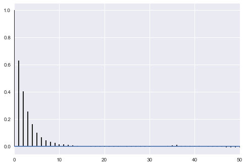
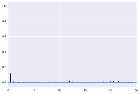
appropriately thinned, we lose any correlation..

def corrplot(trace, maxlags=50):
    plt.acorr(trace-np.mean(trace),  normed=True, maxlags=maxlags);
    plt.xlim([0, maxlags])
corrplot(samps[40000::]);

png

corrplot(samps[40000::5]);

png

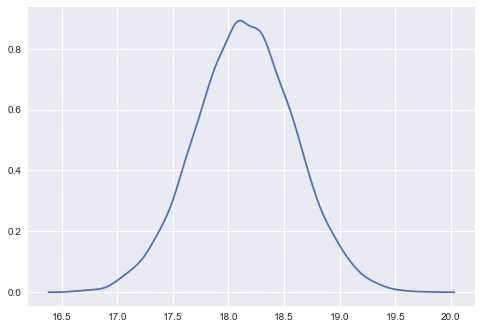
sns.kdeplot(samps[40000::5]);

png

Sampling with pymc

We’ll use this simple example to show how to sample with pymc. To install pymc3, do

conda install -c conda-forge pymc3.

We want pymc 3.3.

Pymc3 is basically a sampler which uses NUTS for continuous variables and Metropolis for discrete ones, but we can force it to use Metropolis for all, which is what we shall do for now.

pymc3 docs are available here.

The structure is that we define a model within a context manager, and optionally do the sampling there. The model name (model1 below) and trace name (model1trace below) are both important names you should keep track of.

The context manager below makes it look as if the variables defined under it do not survive outside the scope of the manager. This is not true, and can be the cause of subtle bugs when comparing models. I would wrap models in functions if you want to keep the variables private.

import pymc3 as pm
with pm.Model() as model1:
    mu = pm.Normal('mu', mu=mu_prior, sd=std_prior)#parameter's prior
    wingspan = pm.Normal('wingspan', mu=mu, sd=np.std(Y), observed=Y)#likelihood
    stepper=pm.Metropolis()
    tracemodel1=pm.sample(100000, step=stepper)

Multiprocess sampling (2 chains in 2 jobs)
Metropolis: [mu]
100%|██████████| 100500/100500 [00:17<00:00, 5595.30it/s]
The number of effective samples is smaller than 25% for some parameters.

Notice that wingspan, which is the data, is defined using the same exact notation as the prior abovem with the addition of the observed argument. This is because Bayesian notation does not distinguish between data d=and parameter nodes..everything is treated equally, and all the action is in taking conditionals and marginals of distributions.

Deterministics are deterministic functions of variables:

model1.deterministics

[]

The variables:

model1.vars, model1.named_vars, type(model1.mu)

([mu], {'mu': mu, 'wingspan': wingspan}, pymc3.model.FreeRV)

The “Observed” Variables, or data.

model1.observed_RVs, type(model1.wingspan)

([wingspan], pymc3.model.ObservedRV)

You can sample from stochastics

model1.mu.random(size=10)

array([ 17.32474626,  29.50049617,  26.45924045,  12.24361447,
        26.43876385,  14.00794413,  26.90755711,  13.93294996,
        21.79692203,   5.10960527])

And key for metropolis or other sampling algorithms, you must be able to get a log-probability for anything that has a distribution

model1.mu.logp({mu: '20'})

array(-3.2227736261987188)

Results

Pymc3 gives us a nice summary of our trace

pm.summary(tracemodel1[50000::])

	mean	sd	mc_error	hpd_2.5	hpd_97.5	n_eff	Rhat
mu	18.147083	0.44278	0.002866	17.298008	19.039121	22355.0	0.999995

The highest-posterior-density is the smallest width interval containing a pre-specified density amount. Here the default is the smallest width containing 95% of the density. Such an interval is called a Bayesian Credible Interval.

pm.hpd(tracemodel1[50000::])#pm.hpd(tracemodel1, alpha=0.05)

{0: {'mu': array([ 17.28695356,  19.03233939])},
 1: {'mu': array([ 17.29833448,  19.03235383])}}

You can also get quantiles:

pm.quantiles(tracemodel1[50000::])

{0: {'mu': {2.5: 17.265736808303036,
17.848775969286105,
18.146892529315949,
18.443961797420624,
5: 19.015918935487345}},
{'mu': {2.5: 17.277567461536957,
17.848590057615525,
18.149979736301887,
18.442791702077095,
5: 19.016768181085421}}}

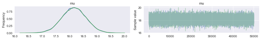
pm.traceplot will give you marginal posteriors and traces for all the “stochastics” in your model (ie non-data). It can even give you traces for some deterministic functions of stochastics..we shall see an example of this soon.

pm.traceplot(tracemodel1[50000::]);

png

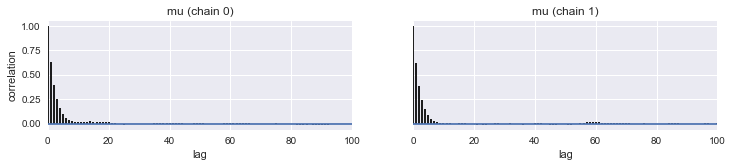
Autocorrelation is easily accessible as well.

pm.autocorrplot(tracemodel1[50000::]);

png

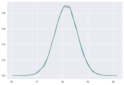
Here we plot the results of our sampling against our manual sampler and see that all three match well.

sns.kdeplot(samps[50000::]);
sns.kdeplot(tracemodel1[50000::]['mu']);

png

The posterior predictive is accessed via the sample_ppc function, which takes the trace, the number of samples wanted, and the model as arguments. The sampler will use the posterior traces and the defined likelihood to return samples from the posterior predictive.

tr1 = tracemodel1[50000::]
postpred = pm.sample_ppc(tr1, 1000, model1)

100%|██████████| 1000/1000 [00:00<00:00, 3755.56it/s]

The posterior predictive will return samples for all data in the model’s observed_RVs.

model1.observed_RVs

[wingspan]

postpred['wingspan'][:10]

array([ 18.82984231,  17.78409678,  18.98763532,  17.70567857,
        20.01378735,  19.41124152,  17.40958767,  19.24012935,
        19.65615391,  19.56344576])

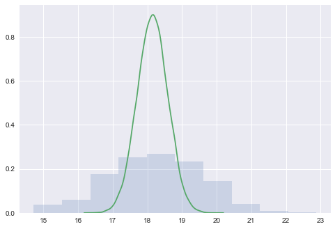
We plot the posterior predictive against the posterior to see how it is spread out! When we compare the posterior predictive to the posterior (unlike in the beta-binomial distribution where one is a rate and one is a count, here both are on the same scale), we find that the posterior predictive is smeared out due to the additional uncertainty from the sampling distribution.

plt.hist(postpred['wingspan'], alpha=0.2, normed=True)
sns.kdeplot(tr1['mu']);

png

Letting $\sigma$ be a stochastic

with pm.Model() as model12:
    mu = pm.Normal('mu', mu=mu_prior, sd=std_prior)#parameter's prior
    sigma = pm.Uniform('sigma', lower=0, upper=10)
    wingspan = pm.Normal('wingspan', mu=mu, sd=sigma, observed=Y)#likelihood
    stepper=pm.Metropolis()
    tracemodel2=pm.sample(100000, step=stepper)

Multiprocess sampling (2 chains in 2 jobs)
CompoundStep
>Metropolis: [sigma_interval__]
>Metropolis: [mu]
100%|██████████| 100500/100500 [00:59<00:00, 1683.49it/s]
The number of effective samples is smaller than 25% for some parameters.

Few things to notice:

the model being implemented is simply:

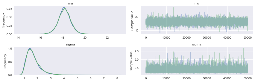
$h \sim N(\mu, \sigma)\\ \mu \sim Normal(\mu_{prior}, \sigma_{prior})\\ \sigma \sim Unif(0, 10)$

we dont have to write log probs or even a proposal. A normal is standardly used.

pm.traceplot(tracemodel2[50000::])

array([[<matplotlib.axes._subplots.AxesSubplot object at 0x110ee7320>,
        <matplotlib.axes._subplots.AxesSubplot object at 0x1112cdf60>],
       [<matplotlib.axes._subplots.AxesSubplot object at 0x110eed5f8>,
        <matplotlib.axes._subplots.AxesSubplot object at 0x11137ac88>]], dtype=object)

png

pm.summary(tracemodel2[50000::])

	mean	sd	mc_error	hpd_2.5	hpd_97.5	n_eff	Rhat
mu	18.150133	0.592374	0.003492	16.931460	19.305538	20373.0	1.000159
sigma	1.700801	0.548500	0.004664	0.897263	2.774750	13294.0	1.000132

model12.vars

[mu, sigma_interval__]

model12.mu.logp(dict(mu=20, sigma_interval__=1))

array(-3.2227736261987188)

model12.sigma_interval__.logp(dict(mu=20, sigma_interval__=1))

array(-1.626523343061009)