The normal model

Keywords: bayesian | normal-normal model | conjugate prior | Download Notebook

Normal Model for fixed $\sigma$
Example of the normal model for fixed $\sigma$

%matplotlib inline
import numpy as np
import matplotlib.pylab as plt 
import seaborn as sn

from scipy.stats import norm

A random variable $Y$ is normally distributed with mean $\mu$ and variance $\sigma^2$. Thus its density is given by :

$p(y \vert \mu, \sigma^2) = \frac{1}{ \sqrt{ 2 \pi \sigma^2}} e^{-( \frac{y-\mu}{2 \sigma})^2}$

Suppose our model is ${y_1, \ldots, y_n \vert \mu, \sigma^2 } \sim N(\mu, \sigma^2)$ then the likelihood is

$p(y_1, \ldots, y_n \vert \mu, \sigma^2) = \prod_{i=1}^{n} p(y_i \vert \mu, \sigma^2)=\prod_{i=1}^{n} \frac{1}{ \sqrt{ 2 \pi \sigma^2}} e^{-( \frac{(y_i-\mu)^2}{2\sigma^2})} = \frac{1}{ \sqrt{ 2 \pi \sigma^2}} \exp \left\{ - \frac{1}{2} \sum_i \frac{(y_i-\mu)^2}{\sigma^2} \right\}$

We can now write the posterior for this model thus:

$p( \mu, \sigma^2 \vert y_1, \ldots, y_n, \sigma^2) \propto \frac{1}{ \sqrt{ 2 \pi \sigma^2}} e^{ - \frac{1}{2\sigma^2} \sum (y_i - \mu)^2 } \, p(\mu, \sigma^2)$

Lets see the posterior of $\mu$ assuming we know $\sigma^2$.

Normal Model for fixed $\sigma$

Now we wish to condition on a known $\sigma^2$. The prior probability distribution for it can then be written as:

$p(\sigma^2) = \delta(\sigma^2 -\sigma_0^2)$

(which does integrate to 1).

Now, keeping in mind that $p(\mu, \sigma^2) = p(\mu \vert \sigma^2) p(\sigma^2)$ and carrying out the integral over $\sigma^2$ which because of the delta distribution means that we must just substitute $\sigma_0^2$ in, we get:

$p( \mu \vert y_1, \ldots, y_n, \sigma^2 = \sigma_0^2) \propto p(\mu \vert \sigma^2=\sigma_0^2) \,e^{ - \frac{1}{2\sigma_0^2} \sum (y_i - \mu)^2 }$

where I have dropped the $\frac{1}{\sqrt{2\pi\sigma_0^2}}$ factor as there is no stochasticity in it (its fixed).

Say we have the prior

$p(\mu \vert \sigma^2) = \exp \left\{ -\frac{1}{2 \tau^2} (\hat{\mu}-\mu)^2 \right\}$

then it can be shown that the posterior is

$p( \mu \vert y_1, \ldots, y_n, \sigma^2) \propto \exp \left\{ -\frac{a}{2} (\mu-b/a)^2 \right\}$ where $a = \frac{1}{\tau^2} + \frac{n}{\sigma_0^2} , \;\;\;\;\; b = \frac{\hat{\mu}}{\tau^2} + \frac{\sum y_i}{\sigma_0^2}$ This is a normal density curve with $1/\sqrt{a}$ playing the role of the standard deviation and $b/a$ playing the role of the mean. Re-writing this,

$p( \mu \vert y_1, \ldots, y_n, \sigma^2) \propto \exp\left\{ -\frac{1}{2} \left( \frac{\mu-b/a}{1/\sqrt(a)}\right)^2 \right\}$

The conjugate of the normal is the normal itself.

Define $\kappa = \sigma^2 / \tau^2 $ to be the variance of the sample model in units of variance of our prior belief (prior distribution) then the posterior mean is

$\mu_p = \frac{b}{a} = \frac{ \kappa}{\kappa + n } \hat{\mu} + \frac{n}{\kappa + n} \bar{y}$

which is a weighted average of prior mean and sampling mean. The variance is

$\sigma_p^2 = \frac{1}{1/\tau^2+n/\sigma^2}$ or better

$\frac{1}{\sigma_p^2} = \frac{1}{\tau^2} + \frac{n}{\sigma^2}.$

You can see that as $n$ increases, the data dominates the prior and the posterior mean approaches the data mean, with the posterior distribution narrowing…

Example of the normal model for fixed $\sigma$

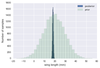
We have data on the wing length in millimeters of a nine members of a particular species of moth. We wish to make inferences from those measurements on the population mean $\mu$. Other studies show the wing length to be around 19 mm. We also know that the length must be positive. We can choose a prior that is normal and most of the density is above zero ($\mu=19.5,\tau=10$). This is only a marginally informative prior.

Many bayesians would prefer you choose relatively uninformative (and thus weakly regularizing) priors. This keeps the posterior in-line (it really does help a sampler remain in important regions), but does not add too much information into the problem.

The measurements were: 16.4, 17.0, 17.2, 17.4, 18.2, 18.2, 18.2, 19.9, 20.8 giving $\bar{y}=18.14$.

Y = [16.4, 17.0, 17.2, 17.4, 18.2, 18.2, 18.2, 19.9, 20.8]
#Data Quantities
sig = np.std(Y) # assume that is the value of KNOWN sigma (in the likelihood)
mu_data = np.mean(Y)
n = len(Y)
print("sigma", sig, "mu", mu_data, "n", n)

sigma 1.33092374864 mu 18.1444444444 n 9

# Prior mean
mu_prior = 19.5
# prior std
tau = 10 

kappa = sig**2 / tau**2
sig_post =np.sqrt(1./( 1./tau**2 + n/sig**2));
# posterior mean
mu_post = kappa / (kappa + n) *mu_prior + n/(kappa+n)* mu_data
print("mu post", mu_post, "sig_post", sig_post)

mu post 18.1471071751 sig_post 0.443205311006

#samples
N = 15000
theta_prior = np.random.normal(loc=mu_prior, scale=tau, size=N);
theta_post = np.random.normal(loc=mu_post, scale=sig_post, size=N);

plt.hist(theta_post, bins=30, alpha=0.9, label="posterior");
plt.hist(theta_prior, bins=30, alpha=0.2, label="prior");
#plt.xlim([10, 30])
plt.xlabel("wing length (mm)")
plt.ylabel("Number of samples")
plt.legend();

png

In the case that we dont know $\sigma^2$ or wont estimate it the way we did above, it turns out that a conjugate prior for the precision (inverse variance) is a gamma distribution. Interested folks can see Murphy’s detailed document here. but you can always just use our MH machinery to draw from any vaguely informative prior for the variance ( a gamma for the precision or even for the variance).

Contents

Contents

Normal Model for fixed $\sigma$

Example of the normal model for fixed $\sigma$