Keywords: normal distribution | multivariate normal | oceanic tools | correlation | covariance | posterior | posterior predictive | gaussian process | poisson regression | Data: Kline2.csv | distmatrix.csv | Download Notebook
Contents
- Reading in our data
- Implementing the simple tools:logpop model and varying intercepts models
- A model with a custom covariance matrix
- Plotting posteriors and predictives
%matplotlib inline
import numpy as np
import scipy as sp
import matplotlib as mpl
import matplotlib.cm as cm
import matplotlib.pyplot as plt
import pandas as pd
pd.set_option('display.width', 500)
pd.set_option('display.max_columns', 100)
pd.set_option('display.notebook_repr_html', True)
import seaborn as sns
sns.set_style("whitegrid")
sns.set_context("poster")
import pymc3 as pm
Reading in our data
We read back the Oceanic tools data
df = pd.read_csv("data/Kline2.csv", sep=';')
df.head()
| culture | population | contact | total_tools | mean_TU | lat | lon | lon2 | logpop | |
|---|---|---|---|---|---|---|---|---|---|
| 0 | Malekula | 1100 | low | 13 | 3.2 | -16.3 | 167.5 | -12.5 | 7.003065 |
| 1 | Tikopia | 1500 | low | 22 | 4.7 | -12.3 | 168.8 | -11.2 | 7.313220 |
| 2 | Santa Cruz | 3600 | low | 24 | 4.0 | -10.7 | 166.0 | -14.0 | 8.188689 |
| 3 | Yap | 4791 | high | 43 | 5.0 | 9.5 | 138.1 | -41.9 | 8.474494 |
| 4 | Lau Fiji | 7400 | high | 33 | 5.0 | -17.7 | 178.1 | -1.9 | 8.909235 |
And center it
df['logpop_c'] = df.logpop - df.logpop.mean()
df.head()
| culture | population | contact | total_tools | mean_TU | lat | lon | lon2 | logpop | logpop_c | |
|---|---|---|---|---|---|---|---|---|---|---|
| 0 | Malekula | 1100 | low | 13 | 3.2 | -16.3 | 167.5 | -12.5 | 7.003065 | -1.973939 |
| 1 | Tikopia | 1500 | low | 22 | 4.7 | -12.3 | 168.8 | -11.2 | 7.313220 | -1.663784 |
| 2 | Santa Cruz | 3600 | low | 24 | 4.0 | -10.7 | 166.0 | -14.0 | 8.188689 | -0.788316 |
| 3 | Yap | 4791 | high | 43 | 5.0 | 9.5 | 138.1 | -41.9 | 8.474494 | -0.502510 |
| 4 | Lau Fiji | 7400 | high | 33 | 5.0 | -17.7 | 178.1 | -1.9 | 8.909235 | -0.067769 |
And read in the distance matrix
dfd = pd.read_csv("data/distmatrix.csv", header=None)
dij=dfd.values
dij
array([[ 0.   ,  0.475,  0.631,  4.363,  1.234,  2.036,  3.178,  2.794,
         1.86 ,  5.678],
       [ 0.475,  0.   ,  0.315,  4.173,  1.236,  2.007,  2.877,  2.67 ,
         1.965,  5.283],
       [ 0.631,  0.315,  0.   ,  3.859,  1.55 ,  1.708,  2.588,  2.356,
         2.279,  5.401],
       [ 4.363,  4.173,  3.859,  0.   ,  5.391,  2.462,  1.555,  1.616,
         6.136,  7.178],
       [ 1.234,  1.236,  1.55 ,  5.391,  0.   ,  3.219,  4.027,  3.906,
         0.763,  4.884],
       [ 2.036,  2.007,  1.708,  2.462,  3.219,  0.   ,  1.801,  0.85 ,
         3.893,  6.653],
       [ 3.178,  2.877,  2.588,  1.555,  4.027,  1.801,  0.   ,  1.213,
         4.789,  5.787],
       [ 2.794,  2.67 ,  2.356,  1.616,  3.906,  0.85 ,  1.213,  0.   ,
         4.622,  6.722],
       [ 1.86 ,  1.965,  2.279,  6.136,  0.763,  3.893,  4.789,  4.622,
         0.   ,  5.037],
       [ 5.678,  5.283,  5.401,  7.178,  4.884,  6.653,  5.787,  6.722,
         5.037,  0.   ]])
Implementing the simple tools:logpop model and varying intercepts models
import theano.tensor as tt
import theano.tensor as t
with pm.Model() as m2c_onlyp:
    betap = pm.Normal("betap", 0, 1)
    alpha = pm.Normal("alpha", 0, 10)
    loglam = alpha + betap*df.logpop_c
    y = pm.Poisson("ntools", mu=t.exp(loglam), observed=df.total_tools)
    trace2c_onlyp = pm.sample(6000, tune=1000)
Auto-assigning NUTS sampler...
Initializing NUTS using jitter+adapt_diag...
Multiprocess sampling (2 chains in 2 jobs)
NUTS: [alpha, betap]
100%|██████████| 7000/7000 [00:05<00:00, 1374.78it/s]
pm.summary(trace2c_onlyp)
| mean | sd | mc_error | hpd_2.5 | hpd_97.5 | n_eff | Rhat | |
|---|---|---|---|---|---|---|---|
| betap | 0.239422 | 0.031505 | 0.000286 | 0.178178 | 0.301947 | 10383.0 | 0.999918 |
| alpha | 3.478431 | 0.057299 | 0.000577 | 3.366003 | 3.587042 | 10055.0 | 0.999939 |
Notice that $\beta_P$ has a value around 0.24
We also implement the varying intercepts per society model from before
with pm.Model() as m3c:
    betap = pm.Normal("betap", 0, 1)
    alpha = pm.Normal("alpha", 0, 10)
    sigmasoc = pm.HalfCauchy("sigmasoc", 1)
    alphasoc = pm.Normal("alphasoc", 0, sigmasoc, shape=df.shape[0])
    loglam = alpha + alphasoc + betap*df.logpop_c
    y = pm.Poisson("ntools", mu=t.exp(loglam), observed=df.total_tools)
with m3c:
    trace3 = pm.sample(6000, tune=1000, nuts_kwargs=dict(target_accept=.95))
Auto-assigning NUTS sampler...
Initializing NUTS using jitter+adapt_diag...
Multiprocess sampling (2 chains in 2 jobs)
NUTS: [alphasoc, sigmasoc_log__, alpha, betap]
100%|██████████| 7000/7000 [00:28<00:00, 247.87it/s]
The number of effective samples is smaller than 25% for some parameters.
pm.summary(trace3)
| mean | sd | mc_error | hpd_2.5 | hpd_97.5 | n_eff | Rhat | |
|---|---|---|---|---|---|---|---|
| betap | 0.258089 | 0.082296 | 0.001338 | 0.096656 | 0.424239 | 4166.0 | 0.999973 |
| alpha | 3.446465 | 0.120746 | 0.002027 | 3.199103 | 3.687472 | 3653.0 | 0.999921 |
| alphasoc__0 | -0.209619 | 0.247940 | 0.003688 | -0.718741 | 0.259506 | 4968.0 | 1.000043 |
| alphasoc__1 | 0.038430 | 0.219664 | 0.002941 | -0.404914 | 0.487200 | 5961.0 | 0.999917 |
| alphasoc__2 | -0.050901 | 0.195434 | 0.002468 | -0.447657 | 0.339753 | 5818.0 | 0.999921 |
| alphasoc__3 | 0.324157 | 0.189557 | 0.002763 | -0.031798 | 0.699002 | 4321.0 | 0.999929 |
| alphasoc__4 | 0.039406 | 0.175986 | 0.002227 | -0.301135 | 0.401451 | 6167.0 | 1.000062 |
| alphasoc__5 | -0.320429 | 0.208348 | 0.003087 | -0.733230 | 0.055638 | 4967.0 | 0.999927 |
| alphasoc__6 | 0.144230 | 0.172236 | 0.002496 | -0.168542 | 0.513625 | 5458.0 | 0.999972 |
| alphasoc__7 | -0.174227 | 0.184070 | 0.002252 | -0.568739 | 0.162993 | 6696.0 | 0.999919 |
| alphasoc__8 | 0.273610 | 0.174185 | 0.002854 | -0.050347 | 0.627762 | 4248.0 | 1.000032 |
| alphasoc__9 | -0.088533 | 0.291865 | 0.004870 | -0.679972 | 0.487844 | 4385.0 | 0.999929 |
| sigmasoc | 0.312019 | 0.129527 | 0.002224 | 0.098244 | 0.588338 | 2907.0 | 0.999981 |
A model with a custom covariance matrix
The assumption here now is that the intercepts for these various societies are correlated…
We use a custom covariance matrix which inverse-square weights distance
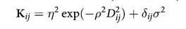
You have seen this before! This is an example of a Gaussian Process Covariance Matrix.
Here is the complete model:
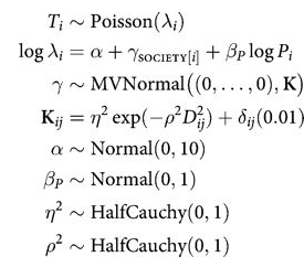
with pm.Model() as mgc:
    betap = pm.Normal("betap", 0, 1)
    alpha = pm.Normal("alpha", 0, 10)
    etasq = pm.HalfCauchy("etasq", 1)
    rhosq = pm.HalfCauchy("rhosq", 1)
    means=tt.stack([0.0]*10)
    sigma_matrix = tt.nlinalg.diag([0.01]*10)
    cov=tt.exp(-rhosq*dij*dij)*etasq + sigma_matrix
    gammasoc = pm.MvNormal("gammasoc", means, cov=cov, shape=df.shape[0])
    loglam = alpha + gammasoc + betap*df.logpop_c
    y = pm.Poisson("ntools", mu=t.exp(loglam), observed=df.total_tools)
with mgc:
    mgctrace = pm.sample(10000, tune=2000, nuts_kwargs=dict(target_accept=.95))
Auto-assigning NUTS sampler...
Initializing NUTS using jitter+adapt_diag...
Multiprocess sampling (2 chains in 2 jobs)
NUTS: [gammasoc, rhosq_log__, etasq_log__, alpha, betap]
100%|██████████| 12000/12000 [05:11<00:00, 38.58it/s]
The acceptance probability does not match the target. It is 0.895944134094, but should be close to 0.8. Try to increase the number of tuning steps.
The number of effective samples is smaller than 25% for some parameters.
pm.summary(mgctrace)
| mean | sd | mc_error | hpd_2.5 | hpd_97.5 | n_eff | Rhat | |
|---|---|---|---|---|---|---|---|
| betap | 0.247414 | 0.116188 | 0.001554 | 0.005191 | 0.474834 | 5471.0 | 1.000157 |
| alpha | 3.512649 | 0.357406 | 0.007140 | 2.790415 | 4.239959 | 2111.0 | 1.001964 |
| gammasoc__0 | -0.269862 | 0.455632 | 0.008620 | -1.239333 | 0.607492 | 2569.0 | 1.001484 |
| gammasoc__1 | -0.117755 | 0.445192 | 0.008520 | -1.041095 | 0.757448 | 2439.0 | 1.001758 |
| gammasoc__2 | -0.165474 | 0.430544 | 0.008116 | -1.042846 | 0.686170 | 2406.0 | 1.001881 |
| gammasoc__3 | 0.299581 | 0.387140 | 0.007481 | -0.481745 | 1.079855 | 2365.0 | 1.001936 |
| gammasoc__4 | 0.026350 | 0.382587 | 0.007425 | -0.763338 | 0.770842 | 2292.0 | 1.001728 |
| gammasoc__5 | -0.458827 | 0.389807 | 0.006976 | -1.286453 | 0.231992 | 2481.0 | 1.001517 |
| gammasoc__6 | 0.097538 | 0.377499 | 0.007064 | -0.653992 | 0.840048 | 2382.0 | 1.001464 |
| gammasoc__7 | -0.263660 | 0.378417 | 0.006917 | -1.077743 | 0.404521 | 2407.0 | 1.001890 |
| gammasoc__8 | 0.233544 | 0.361616 | 0.006715 | -0.510818 | 0.909164 | 2407.0 | 1.001721 |
| gammasoc__9 | -0.123068 | 0.473731 | 0.006671 | -1.034810 | 0.850175 | 3985.0 | 1.000439 |
| etasq | 0.354953 | 0.660893 | 0.009717 | 0.001437 | 1.114851 | 4904.0 | 1.000206 |
| rhosq | 2.306880 | 30.113269 | 0.343453 | 0.000437 | 4.550517 | 8112.0 | 0.999955 |
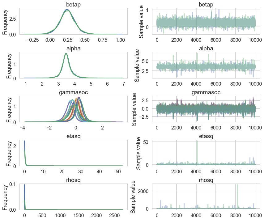
pm.traceplot(mgctrace);
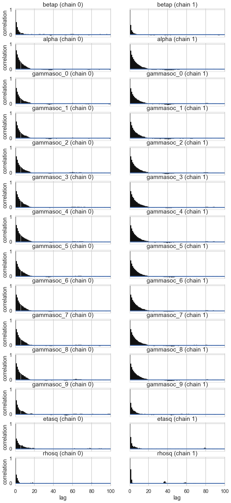
pm.autocorrplot(mgctrace);
d={}
for i, v in enumerate(df.culture.values):
    d[v] = mgctrace['gammasoc'][:,i]
dfsamps=pd.DataFrame.from_dict(d)
dfsamps.head()
| Chuuk | Hawaii | Lau Fiji | Malekula | Manus | Santa Cruz | Tikopia | Tonga | Trobriand | Yap | |
|---|---|---|---|---|---|---|---|---|---|---|
| 0 | 0.282612 | 0.059503 | 0.145726 | -0.024485 | -0.283392 | -0.064665 | 0.211578 | 0.421679 | -0.337896 | 0.552060 |
| 1 | 0.138628 | -0.023895 | 0.202573 | 0.083340 | -0.147399 | 0.037469 | 0.259075 | 0.432713 | -0.513998 | 0.579821 |
| 2 | 0.257026 | 0.065751 | 0.263479 | -0.175381 | -0.196812 | -0.139182 | -0.060890 | 0.358894 | -0.478396 | 0.349795 |
| 3 | 0.138580 | -0.494443 | 0.124155 | 0.065190 | -0.183672 | 0.130431 | 0.207621 | 0.186890 | -0.280590 | 0.541165 |
| 4 | 0.034011 | 0.036418 | 0.224733 | -0.600040 | -0.405896 | -0.531054 | -0.348027 | 0.026920 | -0.589172 | 0.220345 |
dfsamps.describe()
| Chuuk | Hawaii | Lau Fiji | Malekula | Manus | Santa Cruz | Tikopia | Tonga | Trobriand | Yap | |
|---|---|---|---|---|---|---|---|---|---|---|
| count | 20000.000000 | 20000.000000 | 20000.000000 | 20000.000000 | 20000.000000 | 20000.000000 | 20000.000000 | 20000.000000 | 20000.000000 | 20000.000000 |
| mean | 0.097538 | -0.123068 | 0.026350 | -0.269862 | -0.263660 | -0.165474 | -0.117755 | 0.233544 | -0.458827 | 0.299581 |
| std | 0.377509 | 0.473743 | 0.382597 | 0.455644 | 0.378426 | 0.430555 | 0.445203 | 0.361625 | 0.389816 | 0.387149 |
| min | -3.359014 | -3.773198 | -3.389680 | -3.856332 | -3.592680 | -3.704032 | -3.634145 | -3.229867 | -3.808333 | -3.046678 |
| 25% | -0.080201 | -0.369415 | -0.156227 | -0.507103 | -0.444126 | -0.377180 | -0.344367 | 0.064836 | -0.650613 | 0.107982 |
| 50% | 0.108659 | -0.112151 | 0.039389 | -0.242684 | -0.244814 | -0.140033 | -0.098324 | 0.241970 | -0.429267 | 0.304480 |
| 75% | 0.287604 | 0.132445 | 0.220311 | -0.015149 | -0.057941 | 0.070862 | 0.129670 | 0.415369 | -0.233960 | 0.500363 |
| max | 2.908532 | 3.523802 | 2.684128 | 2.373157 | 2.501715 | 2.561251 | 2.619592 | 3.046274 | 2.093728 | 3.017744 |
Plotting posteriors and predictives
Lets plot the covariance posteriors for the 100 random samples in the trace.
smalleta=np.random.choice(mgctrace['etasq'], replace=False, size=100)
smallrho=np.random.choice(mgctrace['rhosq'], replace=False, size=100)
with sns.plotting_context('poster'):
    d=np.linspace(0,10,100)
    for i in range(100):
        covarod = lambda d: smalleta[i]*np.exp(-smallrho[i]*d*d)
        plt.plot(d, covarod(d),alpha=0.1, color='k')
    medetasq=np.median(mgctrace['etasq'])
    medrhosq=np.median(mgctrace['rhosq'])
    covarodmed = lambda d: medetasq*np.exp(-medrhosq*d*d)
    plt.plot(d, covarodmed(d),alpha=1.0, color='k', lw=3)
    plt.ylim([0,1]);
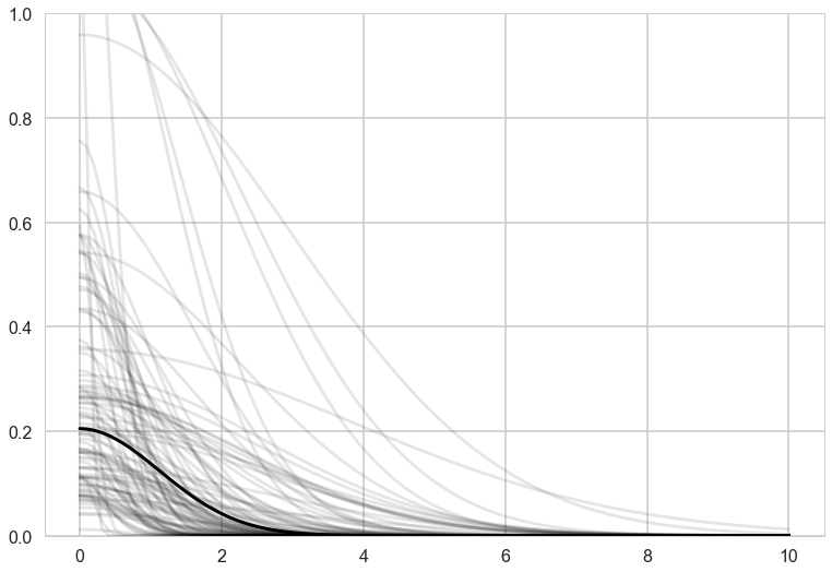
The x-axis is thousands of kilometers. Notice how almost everything damps out by 4000 kms. Lets calculate the median correlation matrix:
medkij = np.diag([0.01]*10)+medetasq*(np.exp(-medrhosq*dij*dij))
#from statsmodels
def cov2corr(cov, return_std=False):
    '''convert covariance matrix to correlation matrix

    Parameters
    ----------
    cov : array_like, 2d
        covariance matrix, see Notes

    Returns
    -------
    corr : ndarray (subclass)
        correlation matrix
    return_std : bool
        If this is true then the standard deviation is also returned.
        By default only the correlation matrix is returned.

    Notes
    -----
    This function does not convert subclasses of ndarrays. This requires
    that division is defined elementwise. np.ma.array and np.matrix are allowed.

    '''
    cov = np.asanyarray(cov)
    std_ = np.sqrt(np.diag(cov))
    corr = cov / np.outer(std_, std_)
    if return_std:
        return corr, std_
    else:
        return corr
medcorrij=cov2corr(medkij)
medcorrij
array([[  1.00000000e+00,   8.71785980e-01,   8.14096714e-01,
          4.99776683e-04,   5.21038310e-01,   1.84041573e-01,
          1.73288749e-02,   4.30502586e-02,   2.41593313e-01,
          2.65025654e-06],
       [  8.71785980e-01,   1.00000000e+00,   9.16627626e-01,
          9.51206322e-04,   5.20017938e-01,   1.92806478e-01,
          3.57157022e-02,   5.63298362e-02,   2.06001853e-01,
          1.47715424e-05],
       [  8.14096714e-01,   9.16627626e-01,   1.00000000e+00,
          2.58767794e-03,   3.67501866e-01,   2.99604292e-01,
          6.68407750e-02,   1.05368392e-01,   1.21399142e-01,
          8.95698536e-06],
       [  4.99776683e-04,   9.51206322e-04,   2.58767794e-03,
          1.00000000e+00,   9.34889296e-06,   8.60394889e-02,
          3.65244813e-01,   3.38258916e-01,   3.09612981e-07,
          1.25890327e-09],
       [  5.21038310e-01,   5.20017938e-01,   3.67501866e-01,
          9.34889296e-06,   1.00000000e+00,   1.56160443e-02,
          1.52965471e-03,   2.23880332e-03,   7.56772084e-01,
          7.38793465e-05],
       [  1.84041573e-01,   1.92806478e-01,   2.99604292e-01,
          8.60394889e-02,   1.56160443e-02,   1.00000000e+00,
          2.63213982e-01,   7.15782789e-01,   2.33071089e-03,
          2.24573987e-08],
       [  1.73288749e-02,   3.57157022e-02,   6.68407750e-02,
          3.65244813e-01,   1.52965471e-03,   2.63213982e-01,
          1.00000000e+00,   5.31771921e-01,   1.06386644e-04,
          1.61407707e-06],
       [  4.30502586e-02,   5.63298362e-02,   1.05368392e-01,
          3.38258916e-01,   2.23880332e-03,   7.15782789e-01,
          5.31771921e-01,   1.00000000e+00,   1.98487950e-04,
          1.55709958e-08],
       [  2.41593313e-01,   2.06001853e-01,   1.21399142e-01,
          3.09612981e-07,   7.56772084e-01,   2.33071089e-03,
          1.06386644e-04,   1.98487950e-04,   1.00000000e+00,
          4.04514877e-05],
       [  2.65025654e-06,   1.47715424e-05,   8.95698536e-06,
          1.25890327e-09,   7.38793465e-05,   2.24573987e-08,
          1.61407707e-06,   1.55709958e-08,   4.04514877e-05,
          1.00000000e+00]])
We’ll data frame it to see clearly
dfcorr = pd.DataFrame(medcorrij*100).set_index(df.culture.values)
dfcorr.columns = df.culture.values
dfcorr
| Malekula | Tikopia | Santa Cruz | Yap | Lau Fiji | Trobriand | Chuuk | Manus | Tonga | Hawaii | |
|---|---|---|---|---|---|---|---|---|---|---|
| Malekula | 100.000000 | 87.178598 | 81.409671 | 4.997767e-02 | 52.103831 | 18.404157 | 1.732887 | 4.305026 | 24.159331 | 2.650257e-04 |
| Tikopia | 87.178598 | 100.000000 | 91.662763 | 9.512063e-02 | 52.001794 | 19.280648 | 3.571570 | 5.632984 | 20.600185 | 1.477154e-03 |
| Santa Cruz | 81.409671 | 91.662763 | 100.000000 | 2.587678e-01 | 36.750187 | 29.960429 | 6.684077 | 10.536839 | 12.139914 | 8.956985e-04 |
| Yap | 0.049978 | 0.095121 | 0.258768 | 1.000000e+02 | 0.000935 | 8.603949 | 36.524481 | 33.825892 | 0.000031 | 1.258903e-07 |
| Lau Fiji | 52.103831 | 52.001794 | 36.750187 | 9.348893e-04 | 100.000000 | 1.561604 | 0.152965 | 0.223880 | 75.677208 | 7.387935e-03 |
| Trobriand | 18.404157 | 19.280648 | 29.960429 | 8.603949e+00 | 1.561604 | 100.000000 | 26.321398 | 71.578279 | 0.233071 | 2.245740e-06 |
| Chuuk | 1.732887 | 3.571570 | 6.684077 | 3.652448e+01 | 0.152965 | 26.321398 | 100.000000 | 53.177192 | 0.010639 | 1.614077e-04 |
| Manus | 4.305026 | 5.632984 | 10.536839 | 3.382589e+01 | 0.223880 | 71.578279 | 53.177192 | 100.000000 | 0.019849 | 1.557100e-06 |
| Tonga | 24.159331 | 20.600185 | 12.139914 | 3.096130e-05 | 75.677208 | 0.233071 | 0.010639 | 0.019849 | 100.000000 | 4.045149e-03 |
| Hawaii | 0.000265 | 0.001477 | 0.000896 | 1.258903e-07 | 0.007388 | 0.000002 | 0.000161 | 0.000002 | 0.004045 | 1.000000e+02 |
Notice how there is correlation in the upper left and with Manus and Trobriand. Mcelreath has a distance plot i reproduce below:
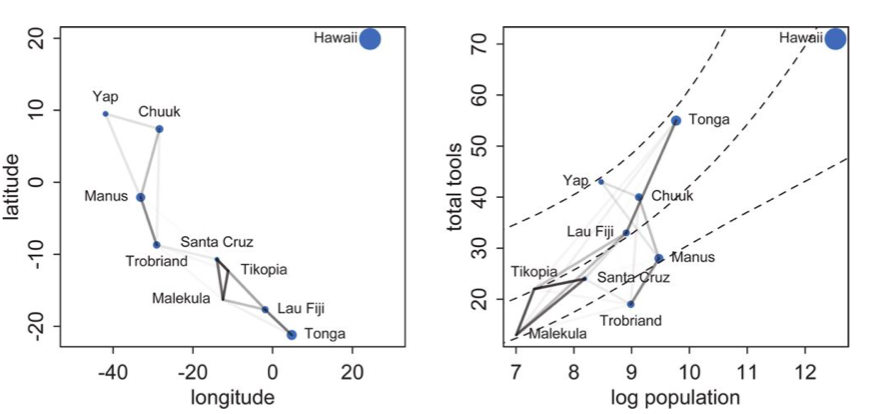
To produce a plot like the one on the right, we calculate the posterior predictives with the correlation free part of the model and then overlay the correlations
from scipy.stats import poisson
def compute_pp_no_corr(lpgrid, trace, contact=0):
    alphatrace = trace['alpha']
    betaptrace = trace['betap']
    tl=len(trace)
    gl=lpgrid.shape[0]
    lam = np.empty((gl, 2*tl))
    lpgrid = lpgrid - lpgrid.mean()
    for i, v in enumerate(lpgrid):
        temp = alphatrace + betaptrace*lpgrid[i]
        lam[i,:] = poisson.rvs(np.exp(temp))
    return lam
lpgrid = np.linspace(6,13,30)
pp = compute_pp_no_corr(lpgrid, mgctrace)
ppmed = np.median(pp, axis=1)
pphpd = pm.stats.hpd(pp.T)
import itertools
corrs={}
for i, j in itertools.product(range(10), range(10)):
    if i <j:
        corrs[(i,j)]=medcorrij[i,j]
corrs
{(0, 1): 0.87178598035086485,
 (0, 2): 0.81409671378956938,
 (0, 3): 0.00049977668270061984,
 (0, 4): 0.52103830967748688,
 (0, 5): 0.18404157314186861,
 (0, 6): 0.017328874910928813,
 (0, 7): 0.04305025856741021,
 (0, 8): 0.241593313072233,
 (0, 9): 2.6502565440185815e-06,
 (1, 2): 0.9166276258652174,
 (1, 3): 0.00095120632192379471,
 (1, 4): 0.5200179376567835,
 (1, 5): 0.19280647828541175,
 (1, 6): 0.035715702211517139,
 (1, 7): 0.05632983623575849,
 (1, 8): 0.20600185316804365,
 (1, 9): 1.4771542363619412e-05,
 (2, 3): 0.0025876779443579313,
 (2, 4): 0.36750186564264986,
 (2, 5): 0.29960429169647806,
 (2, 6): 0.066840774961541019,
 (2, 7): 0.10536839180821188,
 (2, 8): 0.12139914234488278,
 (2, 9): 8.9569853640368644e-06,
 (3, 4): 9.348892959453282e-06,
 (3, 5): 0.086039488876625755,
 (3, 6): 0.36524481329909764,
 (3, 7): 0.33825891559247928,
 (3, 8): 3.0961298086947269e-07,
 (3, 9): 1.2589032666550904e-09,
 (4, 5): 0.01561604425648749,
 (4, 6): 0.0015296547115497437,
 (4, 7): 0.0022388033209531861,
 (4, 8): 0.75677208354568837,
 (4, 9): 7.3879346458710708e-05,
 (5, 6): 0.26321398249820332,
 (5, 7): 0.71578278931845729,
 (5, 8): 0.0023307108876489215,
 (5, 9): 2.2457398672039314e-08,
 (6, 7): 0.53177192062078238,
 (6, 8): 0.00010638664384256532,
 (6, 9): 1.6140770654271327e-06,
 (7, 8): 0.00019848794950225336,
 (7, 9): 1.557099581470421e-08,
 (8, 9): 4.0451487726182869e-05}
with sns.plotting_context('poster'):
    plt.plot(df.logpop, df.total_tools,'o', color="g")
    lpv = df.logpop.values
    ttv = df.total_tools.values
    for a,x,y in zip(df.culture.values, lpv, ttv):
        plt.annotate(a, xy=(x,y))
    for i in range(10):
        for j in range(10):
            if i < j:
                plt.plot([lpv[i],lpv[j]],[ttv[i], ttv[j]],'k', alpha=corrs[(i,j)]/1.)
    plt.plot(lpgrid, ppmed, color="g")
    plt.fill_between(lpgrid, pphpd[:,0], pphpd[:,1], color="g", alpha=0.2, lw=1)
    plt.ylim([10, 75])
    plt.xlim([6.5, 13])
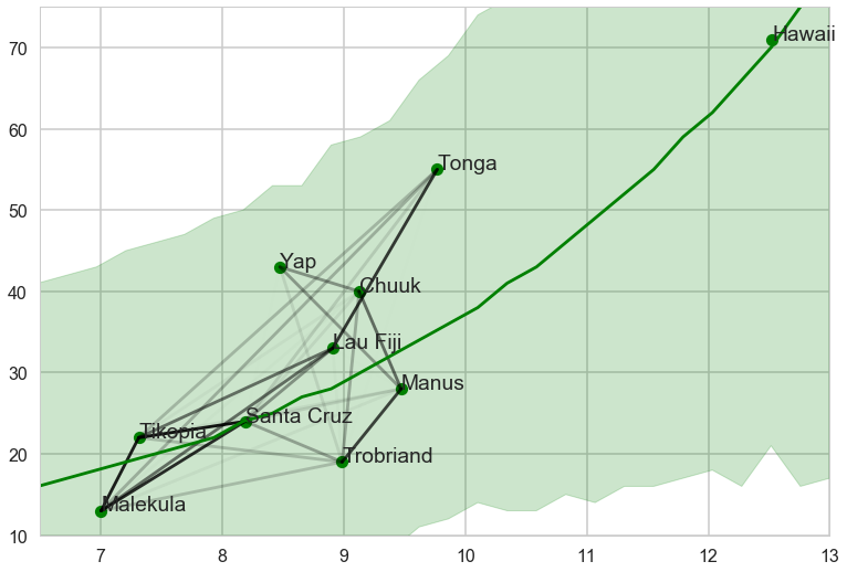
Notice how distance probably pulls Fiji up from the median, and how Manus and Trobriand are below the median but highly correlated. A smaller effect can be seen with the triangle on the left. Of-course, causality is uncertain