Distributions

Summary

Remember that a Random Variable is a mapping $ X: \Omega \rightarrow \mathbb{R}$ that assigns a real number $X(\omega)$ to each outcome $\omega$ in a sample space $\Omega$. The definitions below are taken from Larry Wasserman’s All of Statistics.

Cumulative distribution Function

The cumulative distribution function, or the CDF, is a function

$F_X : \mathbb{R} → [0, 1]$ ,

defined by

$F_X (x) = p(X \le x).$

A note on notation: $X$ is a random variable while $x$ is a particular value of the random variable.

Let $X$ be the random variable representing the number of heads in two coin tosses. Then $x$ can take on values 0, 1 and 2. The CDF for this random variable can be drawn thus (taken from All of Stats):

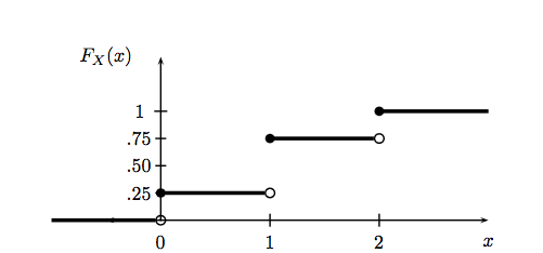
Notice that this function is right-continuous and defined for all $x$, even if $x $does not take real values in-between the integers.

Probability Mass and Distribution Function

$X$ is called a discrete random variable if it takes countably many values ${x_1, x_2,…}$. We define the probability function or the probability mass function (pmf) for X by:

$f_X(x) = p(X=x)$

$f_X$ is a probability.

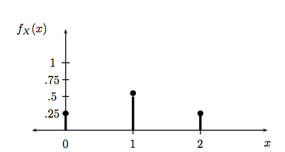
The pmf for the number of heads in two coin tosses (taken from All of Stats) looks like this:

On the other hand, a random variable is called a continuous random variable if there exists a function $f_X$ such that $f_X (x) \ge 0$ for all x, $\int_{-\infty}^{\infty} f_X (x) dx = 1$ and for every a ≤ b,

$p(a < X < b) = \int_{a}^{b} f_X (x) dx$

The function $f_X$ is called the probability density function (pdf). We have the CDF:

$F_X (x) = \int_{-\infty}^{x}f_X (t) dt$

and $f_X (x) = \frac{d F_X (x)}{dx}$ at all points x at which $F_X$ is differentiable.

Continuous variables are confusing. Note:

$p(X=x) = 0$ for every $x$. You cant think of $f_X(x)$ as $p(X=x)$. This holds only for discretes. You can only get probabilities from a pdf by integrating, if only over a very small paty of the space.
A pdf can be bigger than 1 unlike a probability mass function, since probability masses represent actual probabilities.

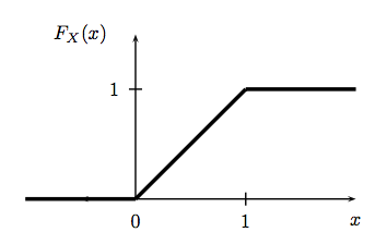
A continuous example: the Uniform Distribution

Suppose that X has pdf $f_X (x) = \begin{cases} 1 & \text{for } 0 \leq x\leq 1\\ 0 & \text{otherwise.} \end{cases}$ A random variable with this density is said to have a Uniform (0,1) distribution. This is meant to capture the idea of choosing a point at random between 0 and 1. The cdf is given by: $F_X (x) = \begin{cases} 0 & x \le 0\\ x & 0 \leq x \leq 1\\ 1 & x > 1. \end{cases}$ and can be visualized as so (again from All of Stats):

A discrete example: the Bernoulli Distribution

The Bernoulli Distribution represents the distribution a coin flip. Let the random variable $X$ represent such a coin flip, where $X=1$ is heads, and $X=0$ is tails. Let us further say that the probability of heads is $p$ ($p=0.5$ is a fair coin).

We then say:

$X \sim Bernoulli(p)$

which is to be read as $X$ has distribution $Bernoulli(p)$. The pmf or probability function associated with the Bernoulli distribution is $f(x) = \begin{cases} 1 - p & x = 0\\ p & x = 1. \end{cases}$

for p in the range 0 to 1. This pmf may be written as

$f(x) = p^x (1-p)^{1-x}$

for x in the set {0,1}.

$p$ is called a parameter of the Bernoulli distribution.

Conditional and Marginal Distributions

Marginal mass functions are defined in analog to probabilities. Thus:

$f_X(x) = p(X=x) = \sum_y f(x, y);\,\, f_Y(y) = p(Y=y) = \sum_x f(x,y).$

Similarly, marginal densities are defined using integrals:

$f_X(x) = \int dy f(x,y);\,\, f_Y(y) = \int dx f(x,y).$

Notice there is no interpretation of the marginal densities in the continuous case as probabilities. An example here if $f(x,y) = e^{-(x+y)}$ defined on the positive quadrant. The marginal is an exponential defined on the positive part of the line.

Conditional mass function is similarly, just a conditional probability. So:

$f_{X \mid Y}(x \mid y) = p(X=x \mid Y=y) = \frac{p(X=x, Y=y)}{p(Y=y)} = \frac{f_{XY}(x,y)}{f_Y(y)}$

The similar formula for continuous densities might be suspected to a bit more complex, because we are conditioning on the event $Y=y$ which strictly speaking has 0 probability. But it can be proved that the same formula holds for densities with some additional requirements and interpretation:

$f_{X \mid Y}(x \mid y) = \frac{f_{XY}(x,y)}{f_Y(y)},$

where we must assume that $f_Y(y) > 0$. Then we have the interpretation that for some event A:

$p(X \in A \mid Y=y) = \int_{x \in A} f_{X \mid Y}(x,y) dx.$

An example of this is the uniform distribution on the unit square. Suppose then that $y=0.3$. Then the conditional density is a uniform density on the line between 0 and 1 at $y=0.3$.