Keywords: box loop |  posterior |  probabilistic modeling | 

Summary

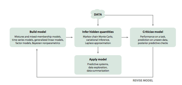
In the 1960’s, the great statistician Box, along with his collaborators, formulated the notion of a loop to understand the nature of the scientific method. This loop is called Box’s loop by Blei et. al., ¹, and illustrated in the diagram (taken from the above linked paper) below:

Box himself focussed on the scientific method, but the loop is applicable at large to other examples of probabilistic modelling, ^[inline note] such as the building of an information retrieval or recommendation system, exploratory data analysis, etc, etc

We:

1. first build a model. This is as much as an art as a science if we are of the philosophical bent that we desire explainability. We bring in domain experts.
2. Using the observed data, we compute the posterior distribution (the distribution of the parameters conditioned on the data) of the (hidden) parameters of the model
3. We then critique our model, studying how they succeed or fail and how they predict future data or on held out sets.
4. If we are satisfied with the performance of our model we apply it in the context of a predictive or explanatory system. If we are not, we go back to 1.