Download Notebook
Contents
- Create some noisy moon shaped data
- Writing a Multi-Layer Perceptron class
- Making a
scikit-learnlike interface - Testing on a wildly overfit model
- Experimentation Space
%matplotlib inline
import numpy as np
import scipy as sp
import matplotlib as mpl
import matplotlib.cm as cm
import matplotlib.pyplot as plt
import pandas as pd
pd.set_option('display.width', 500)
pd.set_option('display.max_columns', 100)
pd.set_option('display.notebook_repr_html', True)
import seaborn.apionly as sns
sns.set_context("poster")
Two additional imports here, seaborn and tqdm. Install via pip or conda
c0=sns.color_palette()[0]
c1=sns.color_palette()[1]
c2=sns.color_palette()[2]
from matplotlib.colors import ListedColormap
cmap_light = ListedColormap(['#FFAAAA', '#AAFFAA', '#AAAAFF'])
cmap_bold = ListedColormap(['#FF0000', '#00FF00', '#0000FF'])
cm = plt.cm.RdBu
cm_bright = ListedColormap(['#FF0000', '#0000FF'])

def points_plot(ax, Xtr, Xte, ytr, yte, clf_predict, colorscale=cmap_light, cdiscrete=cmap_bold, alpha=0.3, psize=20):
    h = .02
    X=np.concatenate((Xtr, Xte))
    x_min, x_max = X[:, 0].min() - .5, X[:, 0].max() + .5
    y_min, y_max = X[:, 1].min() - .5, X[:, 1].max() + .5
    xx, yy = np.meshgrid(np.linspace(x_min, x_max, 100),
                         np.linspace(y_min, y_max, 100))


    Z = clf_predict(np.c_[xx.ravel(), yy.ravel()])
    ZZ = Z.reshape(xx.shape)
    plt.pcolormesh(xx, yy, ZZ, cmap=cmap_light, alpha=alpha, axes=ax)
    showtr = ytr
    showte = yte
    ax.scatter(Xtr[:, 0], Xtr[:, 1], c=showtr-1, cmap=cmap_bold, s=psize, alpha=alpha,edgecolor="k")
    # and testing points
    ax.scatter(Xte[:, 0], Xte[:, 1], c=showte-1, cmap=cmap_bold, alpha=alpha, marker="s", s=psize+10)
    ax.set_xlim(xx.min(), xx.max())
    ax.set_ylim(yy.min(), yy.max())
    return ax,xx,yy
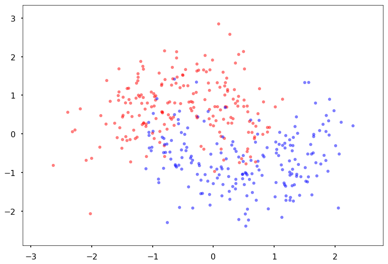
Create some noisy moon shaped data
In order to illustrate classification by a MLP, we first create some noisy moon shaped data. The noise level here and the amount of data is the first thing you might want to experiment with to understand the interplay of amount of data, noise level, number of parameters in the model we use to fit, and overfitting as illustrated by jagged boundaries.
We standardize the data so that it is distributed about 0 as well
from sklearn.datasets import make_moons
from sklearn.model_selection import train_test_split
from sklearn.preprocessing import StandardScaler
dataX, datay = make_moons(noise=0.35, n_samples=400)
dataX = StandardScaler().fit_transform(dataX)
X_train, X_test, y_train, y_test = train_test_split(dataX, datay, test_size=.4)
h=.02
x_min, x_max = dataX[:, 0].min() - .5, dataX[:, 0].max() + .5
y_min, y_max = dataX[:, 1].min() - .5, dataX[:, 1].max() + .5
xx, yy = np.meshgrid(np.arange(x_min, x_max, h),
                     np.arange(y_min, y_max, h))

# just plot the dataset first
cm = plt.cm.RdBu
cm_bright = ListedColormap(['#FF0000', '#0000FF'])
ax = plt.gca()
# Plot the training points
ax.scatter(X_train[:, 0], X_train[:, 1], c=y_train, cmap=cm_bright, alpha=0.5, s=30)
# and testing points
ax.scatter(X_test[:, 0], X_test[:, 1], c=y_test, cmap=cm_bright, alpha=0.5, s=30)
ax.set_xlim(xx.min(), xx.max())
ax.set_ylim(yy.min(), yy.max())
(-2.8829483310505788, 3.3370516689494272)
import torch
import torch.nn as nn
from torch.nn import functional as fn
from torch.autograd import Variable
import torch.utils.data
Writing a Multi-Layer Perceptron class
We wrap the construction of our network
class MLP(nn.Module):
    def __init__(self, input_dim, hidden_dim, output_dim, nonlinearity = fn.tanh, additional_hidden_wide=0):
        super(MLP, self).__init__()
        self.fc_initial = nn.Linear(input_dim, hidden_dim)
        self.fc_mid = nn.ModuleList()
        self.additional_hidden_wide = additional_hidden_wide
        for i in range(self.additional_hidden_wide):
            self.fc_mid.append(nn.Linear(hidden_dim, hidden_dim))
        self.fc_final = nn.Linear(hidden_dim, output_dim)
        self.nonlinearity = nonlinearity

    def forward(self, x):
        x = self.fc_initial(x)
        x = self.nonlinearity(x)
        for i in range(self.additional_hidden_wide):
            x = self.fc_mid[i](x)
            x = self.nonlinearity(x)
        x = self.fc_final(x)
        return x
We use it to train. Notice the double->float casting. Numpy defautlts to double but torch defaulta to float to enable memory efficient GPU usage.
np.dtype(np.float).itemsize, np.dtype(np.double).itemsize
(8, 8)
But torch floats are 4 byte as can be seen from here: http://pytorch.org/docs/master/tensors.html
Training the model
Points to note:
- printing a model prints its layers, handy. Note that we implemented layers as functions. The autodiff graph is constructed on the fly on the first forward pass and used in backward.
- we had to cast to float
model.parametersgives us params,model.named_parameters()gives us assigned names. You can set your own names when you create a layer- we create an iterator over the data, more precisely over batches by doing
iter(loader). This dispatches to the__iter__method of the dataloader. (see https://github.com/pytorch/pytorch/blob/4157562c37c76902c79e7eca275951f3a4b1ef78/torch/utils/data/dataloader.py#L416) Always explore source code to understand what is going on
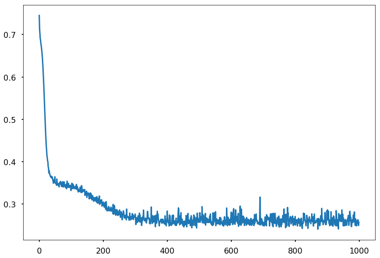
model2 = MLP(input_dim=2, hidden_dim=2, output_dim=2, nonlinearity=fn.tanh, additional_hidden_wide=1)
print(model2)
criterion = nn.CrossEntropyLoss(size_average=True)
dataset = torch.utils.data.TensorDataset(torch.from_numpy(X_train), torch.from_numpy(y_train))
loader = torch.utils.data.DataLoader(dataset, batch_size=64, shuffle=True)
lr, epochs, batch_size = 1e-1 , 1000 , 64
optimizer = torch.optim.SGD(model2.parameters(), lr = lr )
accum=[]
for k in range(epochs):
    localaccum = []
    for localx, localy in iter(loader):
        localx = Variable(localx.float())
        localy = Variable(localy.long())
        output = model2.forward(localx)
        loss = criterion(output, localy)
        model2.zero_grad()
        loss.backward()
        optimizer.step()
        localaccum.append(loss.data[0])
    accum.append(np.mean(localaccum))
plt.plot(accum);
MLP(
  (fc_initial): Linear(in_features=2, out_features=2)
  (fc_mid): ModuleList(
    (0): Linear(in_features=2, out_features=2)
  )
  (fc_final): Linear(in_features=2, out_features=2)
)
The out put from the foward pass is run on the entire test set. Since pytorch tracks layers upto but before the loss, this handily gives us the softmax output, which we can then use np.argmax on.
testoutput = model2.forward(Variable(torch.from_numpy(X_test).float()))
testoutput
Variable containing:
 1.0888 -2.1906
 0.9091 -1.3680
 1.6218 -2.1948
 1.1399 -2.3016
 0.2809 -0.6750
 0.3280 -0.6800
 1.6061 -2.1782
-2.2254  1.9584
 1.4554 -2.1729
-0.0666 -0.2319
 1.7837 -2.3767
 1.6754 -2.2548
 1.5916 -2.1735
 1.4077 -2.4884
-0.5770 -0.1525
-2.5835  2.4284
-2.4546  2.2597
 1.3990 -2.1381
 1.2826 -1.8234
-1.5936  1.5934
-0.4885 -0.3152
 0.9466 -1.4072
 1.4258 -1.9695
 1.3537 -1.8896
-1.7330  1.3134
-1.0528  0.4217
-2.7330  2.6245
-2.0380  1.8422
-0.3440  0.1205
 0.9992 -1.5611
-2.6516  2.5177
 1.4776 -2.2860
-1.1429  0.5401
-2.1433  1.8531
 0.9125 -1.8205
-2.3922  2.1774
-0.1865 -0.0582
 1.0138 -1.4983
 0.6772 -1.5580
 0.2082 -0.5549
-1.0911  0.4734
 0.4373 -1.4409
-1.4554  1.0078
 1.0131 -1.4879
 1.5560 -2.4526
-1.4643  0.9632
 1.6531 -2.4657
-2.2125  1.9458
 0.0266 -0.3921
 0.3066 -0.9172
 0.8946 -2.0540
-1.6135  1.1555
 1.2898 -1.8978
 1.4937 -2.3436
-0.6694  0.3880
 1.9324 -2.8272
 1.7704 -2.3621
-1.6799  1.5354
-2.6629  2.5325
 1.4632 -2.0116
-2.6396  2.5020
 0.6431 -1.2247
 0.0425 -0.9813
 1.3148 -2.4215
-1.5769  1.4020
 1.3001 -1.8268
-2.3835  2.1682
 0.6495 -1.1115
 0.1257 -1.1056
 0.5140 -1.1123
-2.6177  2.4733
-2.1962  1.9228
 1.6184 -2.1932
 1.2048 -1.7866
-1.3650  0.8326
-2.2836  2.0348
 1.2063 -1.7197
-1.6788  1.2537
-1.1056  0.5011
-3.1457  3.3454
-1.0572  0.4265
 1.4560 -2.0427
-2.4383  2.2380
-2.6163  2.4715
-2.0412  1.8878
-0.1216 -0.1927
 1.4471 -1.9958
-0.3093 -0.5423
-1.1629  0.5699
-2.3112  2.0711
-1.2279  1.1772
-0.6104 -0.1304
 1.0999 -1.6006
-0.3166  0.1048
 0.3878 -0.7486
 0.4704 -1.4723
-0.9387  0.3676
-1.2556  0.6860
 0.3199 -0.9532
 1.2597 -1.7929
 1.3754 -2.4566
-2.4075  2.1976
-2.7082  2.7843
-1.0876  0.4733
 0.2338 -0.5501
-0.7243  0.5619
-2.4890  2.3044
 0.7791 -1.2165
 0.4230 -0.9677
-1.7477  1.3316
-1.5916  1.1271
 1.3984 -1.9383
 1.2825 -1.8041
-0.1262 -0.7825
-2.6084  2.4610
-1.3939  1.2871
 0.8304 -1.7092
 0.6022 -1.1540
 0.2422 -1.2522
-0.6504  0.4795
 0.3656 -0.9149
-2.4814  2.2945
-2.0138  2.0698
 0.8826 -1.5214
 0.8444 -1.8043
-2.6256  2.4837
-0.3022  0.0827
-0.6328 -0.1197
 1.1563 -2.3007
-2.2657  2.0113
 1.7901 -2.7866
 0.7806 -1.2439
 1.2393 -1.7619
-2.5057  2.3263
 1.0977 -1.5994
 0.6465 -1.2483
-0.4097 -0.4094
 1.2039 -1.7483
-1.2692  1.0861
 0.8055 -1.8987
-0.2890 -0.5297
 0.6881 -1.1226
-0.8571  0.7612
-1.2951  0.7401
-1.4802  0.9855
-1.0697  0.9834
-1.2449  0.6786
 1.3559 -2.5063
 0.2652 -0.8792
-2.6000  2.4501
-2.2563  1.9990
 1.5835 -2.1525
 1.6417 -2.2194
 1.0297 -2.1999
 0.4252 -1.1855
-1.5052  1.0133
-1.8554  1.7368
-2.4050  2.1942
 1.5036 -2.6023
 1.5179 -2.0762
[torch.FloatTensor of size 160x2]
y_pred = testoutput.data.numpy().argmax(axis=1)
y_pred
array([0, 0, 0, 0, 0, 0, 0, 1, 0, 0, 0, 0, 0, 0, 1, 1, 1, 0, 0, 1, 1, 0, 0,
       0, 1, 1, 1, 1, 1, 0, 1, 0, 1, 1, 0, 1, 1, 0, 0, 0, 1, 0, 1, 0, 0, 1,
       0, 1, 0, 0, 0, 1, 0, 0, 1, 0, 0, 1, 1, 0, 1, 0, 0, 0, 1, 0, 1, 0, 0,
       0, 1, 1, 0, 0, 1, 1, 0, 1, 1, 1, 1, 0, 1, 1, 1, 0, 0, 0, 1, 1, 1, 1,
       0, 1, 0, 0, 1, 1, 0, 0, 0, 1, 1, 1, 0, 1, 1, 0, 0, 1, 1, 0, 0, 0, 1,
       1, 0, 0, 0, 1, 0, 1, 1, 0, 0, 1, 1, 1, 0, 1, 0, 0, 0, 1, 0, 0, 1, 0,
       1, 0, 0, 0, 1, 1, 1, 1, 1, 0, 0, 1, 1, 0, 0, 0, 0, 1, 1, 1, 0, 0])
You can write your own but we import some metrics from sklearn
from sklearn.metrics import confusion_matrix, accuracy_score
confusion_matrix(y_test, y_pred)
array([[75,  5],
       [11, 69]])
accuracy_score(y_test, y_pred)
0.90000000000000002
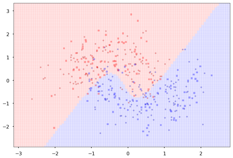
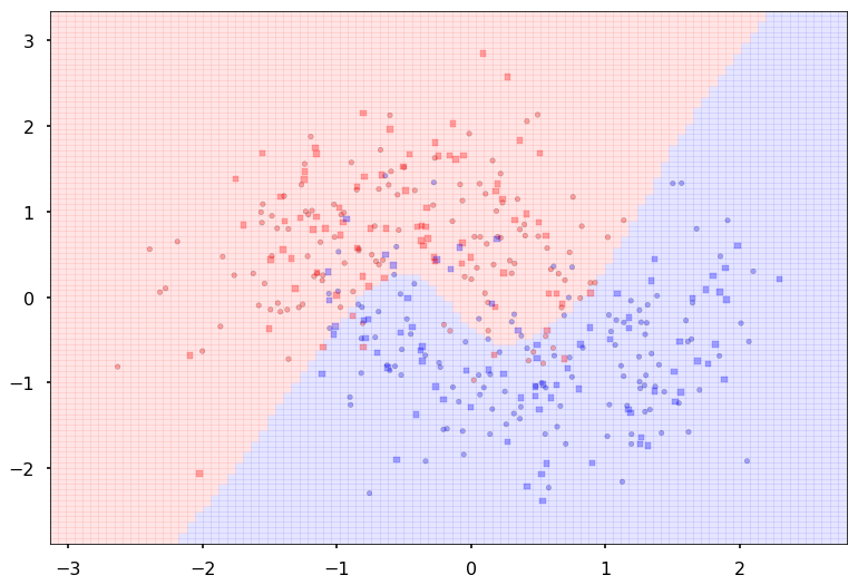
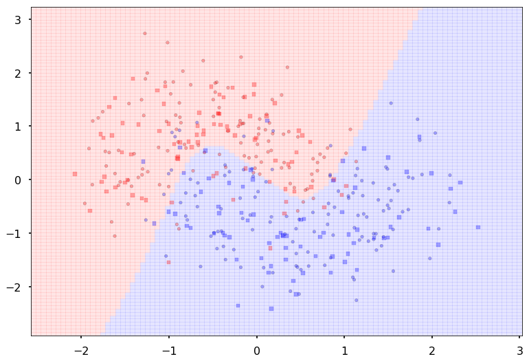
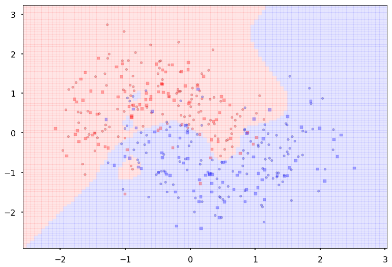
We can wrap this machinery in a function, and pass this function to points_plot to predict on a grid and thus give us a boundary viz
def make_pred(X_set):
    output = model2.forward(Variable(torch.from_numpy(X_set).float()))
    return output.data.numpy().argmax(axis=1)
ax = plt.gca()
points_plot(ax, X_train, X_test, y_train, y_test, make_pred);
Making a scikit-learn like interface
Since we want to run many experiments, we’ll go ahead and wrap our fitting process in a sklearn style interface. Another example of such an interface is here
from tqdm import tnrange, tqdm_notebook
class MLPClassifier:

    def __init__(self, input_dim, hidden_dim,
                 output_dim, nonlinearity = fn.tanh,
                 additional_hidden_wide=0):
        self._pytorch_model = MLP(input_dim, hidden_dim, output_dim, nonlinearity, additional_hidden_wide)
        self._criterion = nn.CrossEntropyLoss(size_average=True)
        self._fit_params = dict(lr=0.1, epochs=200, batch_size=64)
        self._optim = torch.optim.SGD(self._pytorch_model.parameters(), lr = self._fit_params['lr'] )

    def __repr__(self):
        num=0
        for k, p in self._pytorch_model.named_parameters():
            numlist = list(p.data.numpy().shape)
            if len(numlist)==2:
                num += numlist[0]*numlist[1]
            else:
                num+= numlist[0]
        return repr(self._pytorch_model)+"\n"+repr(self._fit_params)+"\nNum Params: {}".format(num)

    def set_fit_params(self, *, lr=0.1, epochs=200, batch_size=64):
        self._fit_params['batch_size'] = batch_size
        self._fit_params['epochs'] = epochs
        self._fit_params['lr'] = lr
        self._optim = torch.optim.SGD(self._pytorch_model.parameters(), lr = self._fit_params['lr'] )

    def fit(self, X_train, y_train):
        dataset = torch.utils.data.TensorDataset(torch.from_numpy(X_train), torch.from_numpy(y_train))
        loader = torch.utils.data.DataLoader(dataset, batch_size=self._fit_params['batch_size'], shuffle=True)
        self._accum=[]
        for k in tnrange(self._fit_params['epochs']):
            localaccum = []
            for localx, localy in iter(loader):
                localx = Variable(localx.float())
                localy = Variable(localy.long())
                output = self._pytorch_model.forward(localx)
                loss = self._criterion(output, localy)
                self._pytorch_model.zero_grad()
                loss.backward()
                self._optim.step()
                localaccum.append(loss.data[0])
            self._accum.append(np.mean(localaccum))

    def plot_loss(self):
        plt.plot(self._accum, label="{}".format(self))
        plt.legend()
        plt.show()

    def plot_boundary(self, X_train, X_test, y_train, y_test):
        points_plot(plt.gca(), X_train, X_test, y_train, y_test, self.predict);
        plt.show()

    def predict(self, X_test):
        output = self._pytorch_model.forward(Variable(torch.from_numpy(X_test).float()))
        return output.data.numpy().argmax(axis=1)
Some points about this:
- we provide the ability to change the fitting parameters
- by implementing a
__repr__we let an instance of this class print something useful. Specifically we created a count of the number of parameters so that we can get a comparison of data size to parameter size.
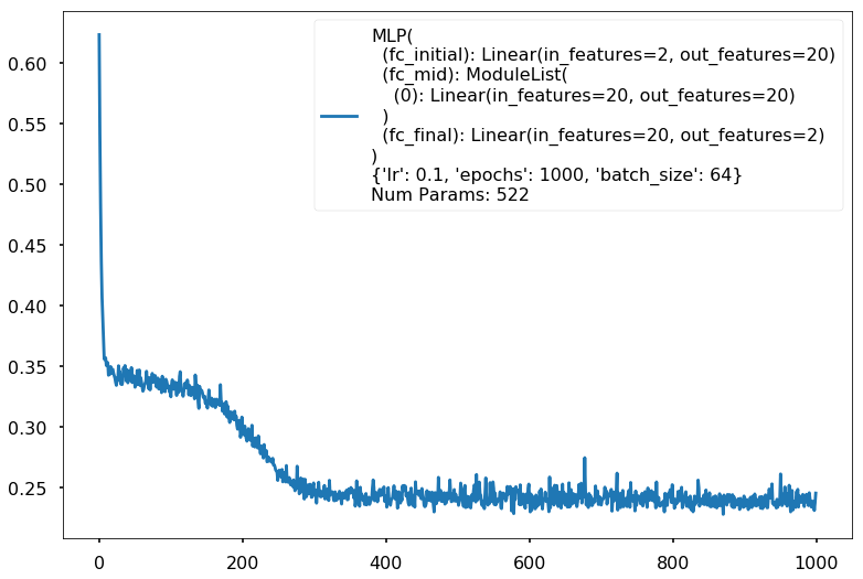
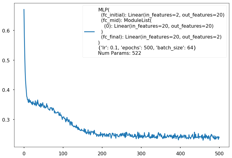
Testing on a wildly overfit model
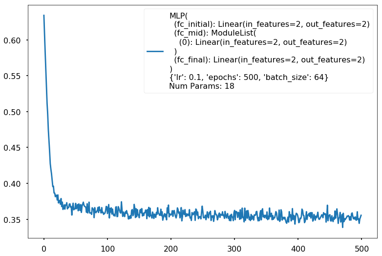
clf = MLPClassifier(input_dim=2, hidden_dim=20, output_dim=2, nonlinearity=fn.tanh, additional_hidden_wide=1)
clf.set_fit_params(epochs=1000)
print(clf)
clf.fit(X_train,y_train)
MLP(
  (fc_initial): Linear(in_features=2, out_features=20)
  (fc_mid): ModuleList(
    (0): Linear(in_features=20, out_features=20)
  )
  (fc_final): Linear(in_features=20, out_features=2)
)
{'lr': 0.1, 'epochs': 1000, 'batch_size': 64}
Num Params: 522
clf.plot_loss()
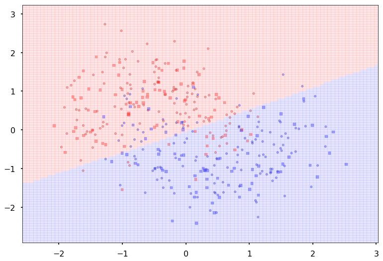
ypred = clf.predict(X_test)
#training and test accuracy
accuracy_score(y_train, clf.predict(X_train)), accuracy_score(y_test, ypred)
(0.89166666666666672, 0.88749999999999996)
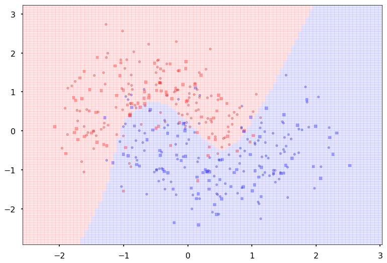
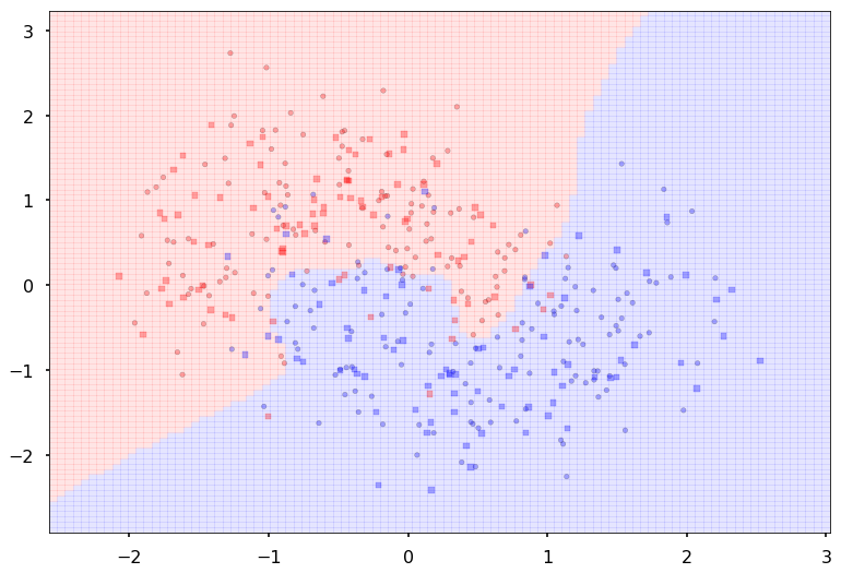
clf.plot_boundary(X_train, X_test, y_train, y_test)
Experimentation Space
Here is space for you to play. You might want to collect accuracies on the traing and test set and plot on a grid of these parameters or some other visualization. Notice how you might want to adjust number of epochs for convergence.
for additional in [1, 2, 3]:
    for hdim in [2, 10, 20, 100, 1000]:
        print('====================')
        print('Additional', additional, "hidden", hdim)
        clf = MLPClassifier(input_dim=2, hidden_dim=hdim, output_dim=2, nonlinearity=fn.tanh, additional_hidden_wide=additional)
        if additional > 2 and hdim > 50:
            clf.set_fit_params(epochs=1000)
        else:
            clf.set_fit_params(epochs=500)
        print(clf)
        clf.fit(X_train,y_train)
        clf.plot_loss()
        clf.plot_boundary(X_train, X_test, y_train, y_test)
        print("Train acc", accuracy_score(y_train, clf.predict(X_train)))
        print("Test acc", accuracy_score(y_test, clf.predict(X_test)))
====================
Additional 1 hidden 2
MLP(
  (fc_initial): Linear(in_features=2, out_features=2)
  (fc_mid): ModuleList(
    (0): Linear(in_features=2, out_features=2)
  )
  (fc_final): Linear(in_features=2, out_features=2)
)
{'lr': 0.1, 'epochs': 500, 'batch_size': 64}
Num Params: 18
Train acc 0.833333333333
Test acc 0.85
====================
Additional 1 hidden 10
MLP(
  (fc_initial): Linear(in_features=2, out_features=10)
  (fc_mid): ModuleList(
    (0): Linear(in_features=10, out_features=10)
  )
  (fc_final): Linear(in_features=10, out_features=2)
)
{'lr': 0.1, 'epochs': 500, 'batch_size': 64}
Num Params: 162
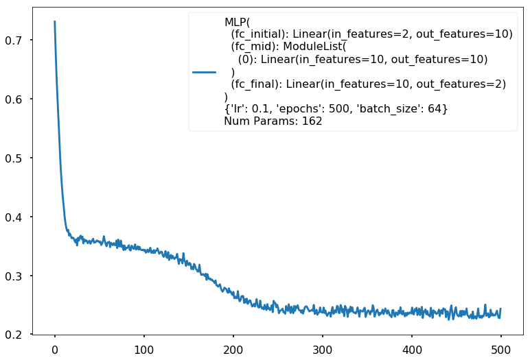

Train acc 0.9
Test acc 0.88125
====================
Additional 1 hidden 20
MLP(
  (fc_initial): Linear(in_features=2, out_features=20)
  (fc_mid): ModuleList(
    (0): Linear(in_features=20, out_features=20)
  )
  (fc_final): Linear(in_features=20, out_features=2)
)
{'lr': 0.1, 'epochs': 500, 'batch_size': 64}
Num Params: 522
Train acc 0.883333333333
Test acc 0.8875
====================
Additional 1 hidden 100
MLP(
  (fc_initial): Linear(in_features=2, out_features=100)
  (fc_mid): ModuleList(
    (0): Linear(in_features=100, out_features=100)
  )
  (fc_final): Linear(in_features=100, out_features=2)
)
{'lr': 0.1, 'epochs': 500, 'batch_size': 64}
Num Params: 10602
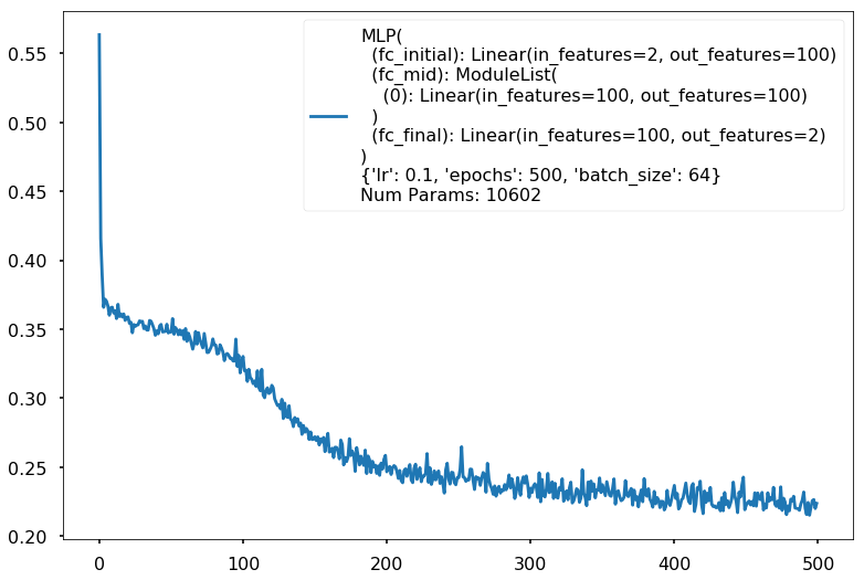
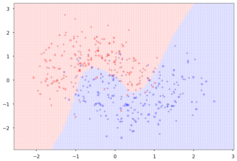
Train acc 0.908333333333
Test acc 0.88125
====================
Additional 1 hidden 1000
MLP(
  (fc_initial): Linear(in_features=2, out_features=1000)
  (fc_mid): ModuleList(
    (0): Linear(in_features=1000, out_features=1000)
  )
  (fc_final): Linear(in_features=1000, out_features=2)
)
{'lr': 0.1, 'epochs': 500, 'batch_size': 64}
Num Params: 1006002
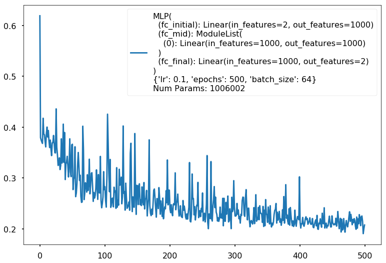
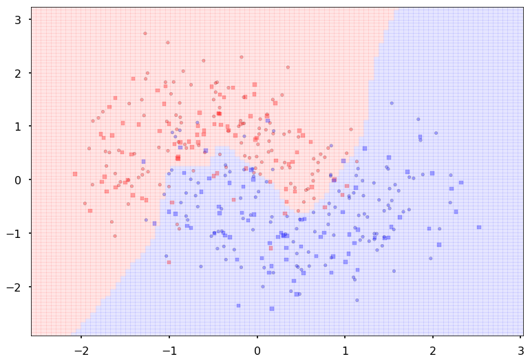
Train acc 0.9125
Test acc 0.88125
====================
Additional 2 hidden 2
MLP(
  (fc_initial): Linear(in_features=2, out_features=2)
  (fc_mid): ModuleList(
    (0): Linear(in_features=2, out_features=2)
    (1): Linear(in_features=2, out_features=2)
  )
  (fc_final): Linear(in_features=2, out_features=2)
)
{'lr': 0.1, 'epochs': 500, 'batch_size': 64}
Num Params: 24
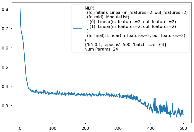
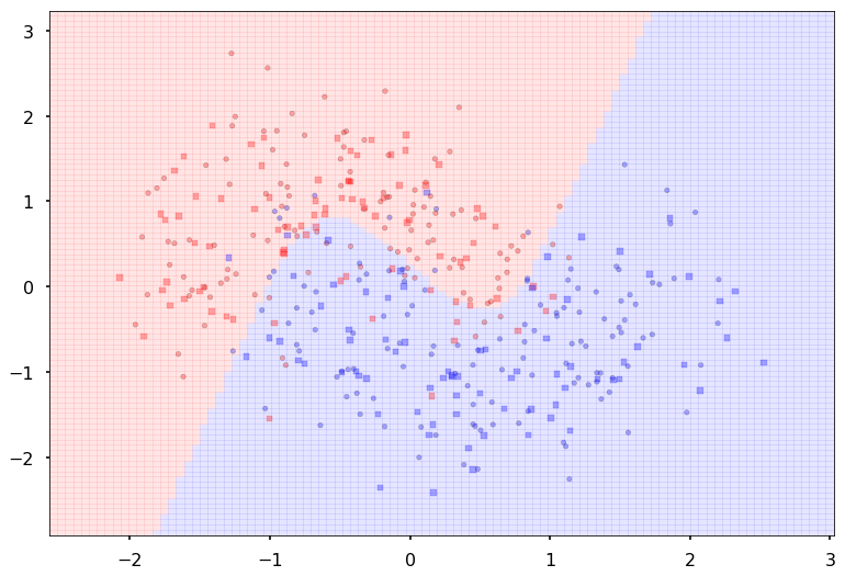
Train acc 0.8875
Test acc 0.875
====================
Additional 2 hidden 10
MLP(
  (fc_initial): Linear(in_features=2, out_features=10)
  (fc_mid): ModuleList(
    (0): Linear(in_features=10, out_features=10)
    (1): Linear(in_features=10, out_features=10)
  )
  (fc_final): Linear(in_features=10, out_features=2)
)
{'lr': 0.1, 'epochs': 500, 'batch_size': 64}
Num Params: 272
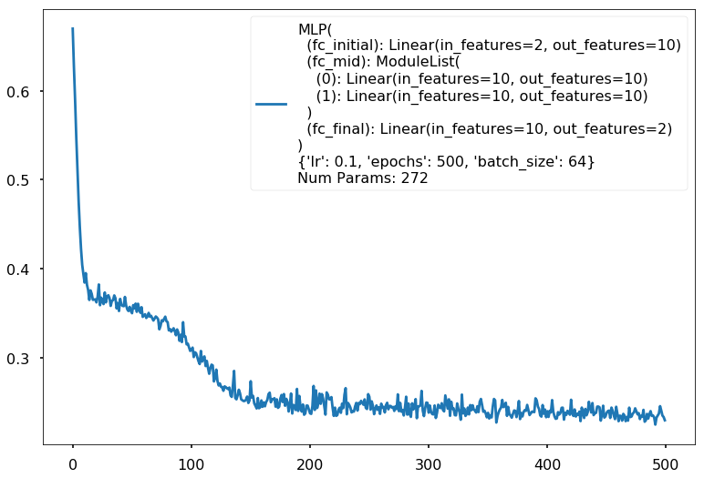
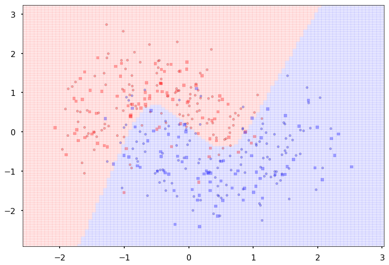
Train acc 0.9
Test acc 0.88125
====================
Additional 2 hidden 20
MLP(
  (fc_initial): Linear(in_features=2, out_features=20)
  (fc_mid): ModuleList(
    (0): Linear(in_features=20, out_features=20)
    (1): Linear(in_features=20, out_features=20)
  )
  (fc_final): Linear(in_features=20, out_features=2)
)
{'lr': 0.1, 'epochs': 500, 'batch_size': 64}
Num Params: 942
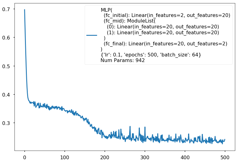
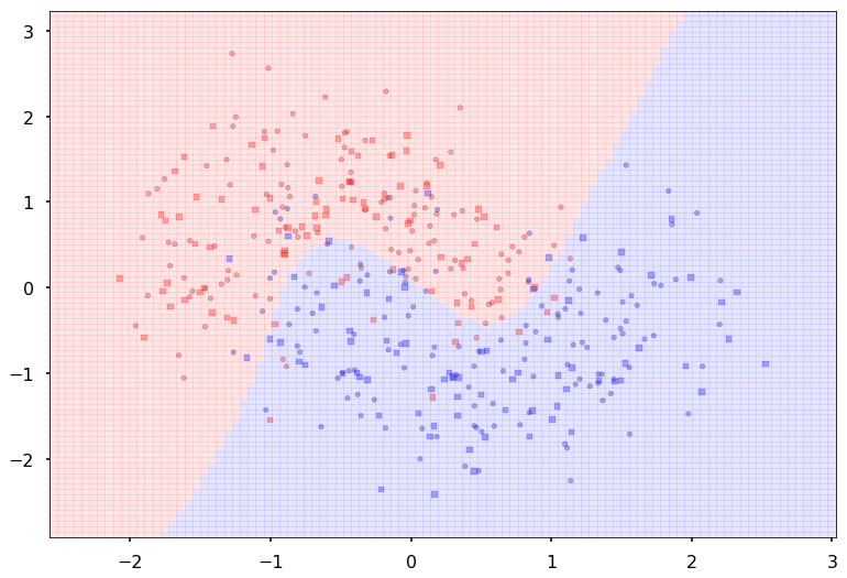
Train acc 0.9
Test acc 0.875
====================
Additional 2 hidden 100
MLP(
  (fc_initial): Linear(in_features=2, out_features=100)
  (fc_mid): ModuleList(
    (0): Linear(in_features=100, out_features=100)
    (1): Linear(in_features=100, out_features=100)
  )
  (fc_final): Linear(in_features=100, out_features=2)
)
{'lr': 0.1, 'epochs': 500, 'batch_size': 64}
Num Params: 20702
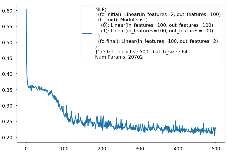
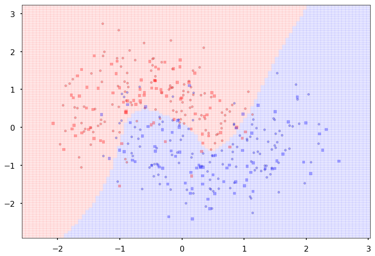
Train acc 0.908333333333
Test acc 0.8875
====================
Additional 2 hidden 1000
MLP(
  (fc_initial): Linear(in_features=2, out_features=1000)
  (fc_mid): ModuleList(
    (0): Linear(in_features=1000, out_features=1000)
    (1): Linear(in_features=1000, out_features=1000)
  )
  (fc_final): Linear(in_features=1000, out_features=2)
)
{'lr': 0.1, 'epochs': 500, 'batch_size': 64}
Num Params: 2007002
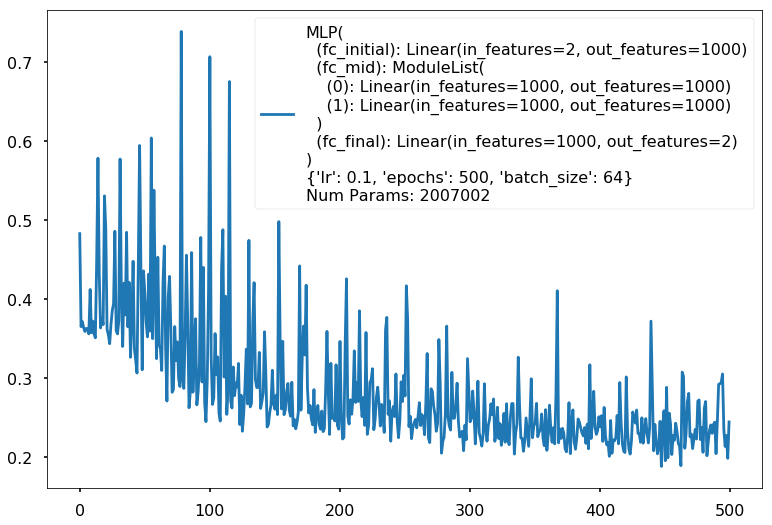
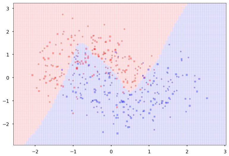
Train acc 0.875
Test acc 0.80625
====================
Additional 3 hidden 2
MLP(
  (fc_initial): Linear(in_features=2, out_features=2)
  (fc_mid): ModuleList(
    (0): Linear(in_features=2, out_features=2)
    (1): Linear(in_features=2, out_features=2)
    (2): Linear(in_features=2, out_features=2)
  )
  (fc_final): Linear(in_features=2, out_features=2)
)
{'lr': 0.1, 'epochs': 500, 'batch_size': 64}
Num Params: 30
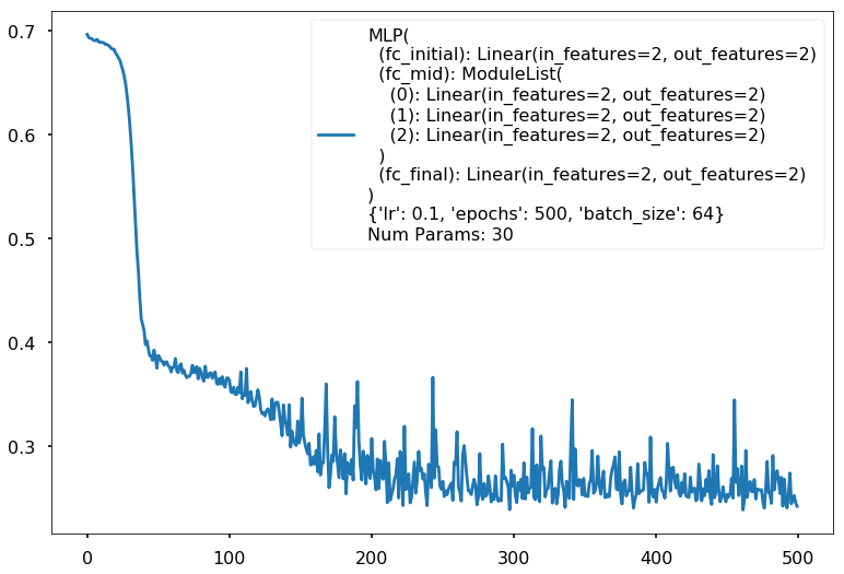
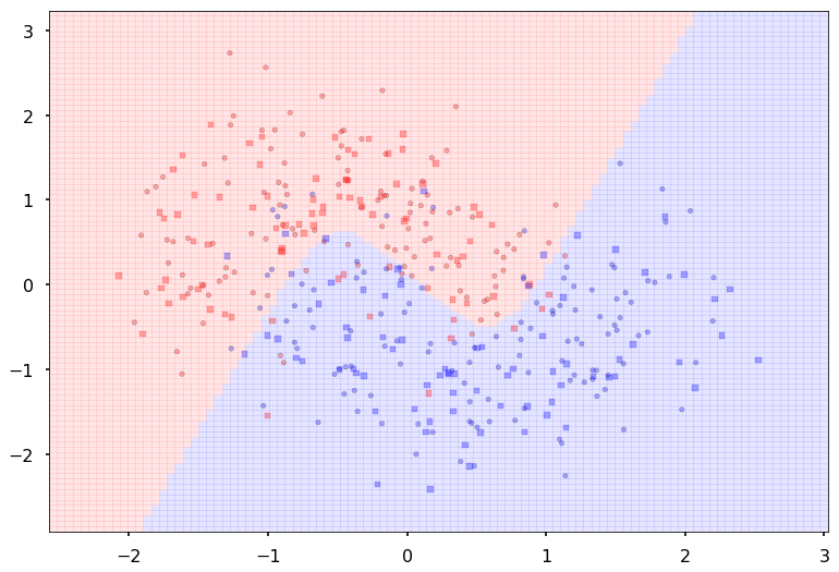
Train acc 0.895833333333
Test acc 0.8875
====================
Additional 3 hidden 10
MLP(
  (fc_initial): Linear(in_features=2, out_features=10)
  (fc_mid): ModuleList(
    (0): Linear(in_features=10, out_features=10)
    (1): Linear(in_features=10, out_features=10)
    (2): Linear(in_features=10, out_features=10)
  )
  (fc_final): Linear(in_features=10, out_features=2)
)
{'lr': 0.1, 'epochs': 500, 'batch_size': 64}
Num Params: 382
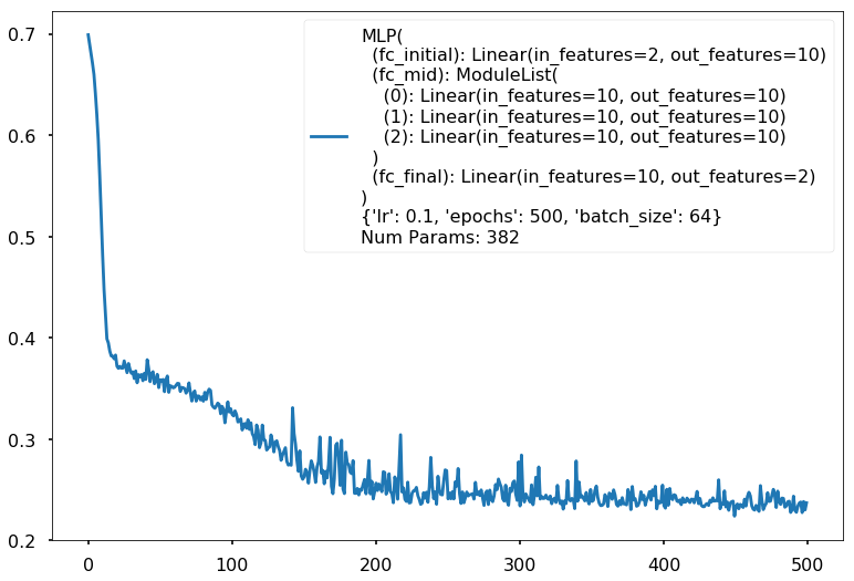
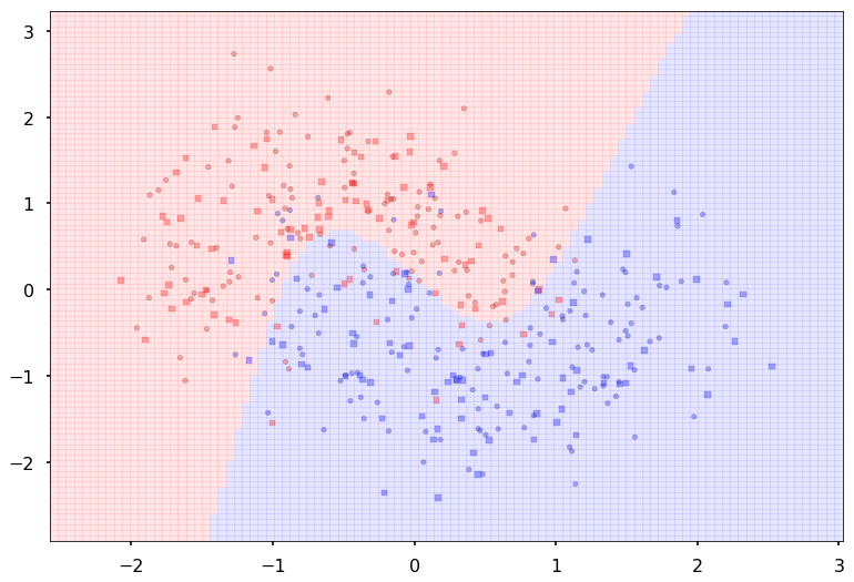
Train acc 0.891666666667
Test acc 0.8875
====================
Additional 3 hidden 20
MLP(
  (fc_initial): Linear(in_features=2, out_features=20)
  (fc_mid): ModuleList(
    (0): Linear(in_features=20, out_features=20)
    (1): Linear(in_features=20, out_features=20)
    (2): Linear(in_features=20, out_features=20)
  )
  (fc_final): Linear(in_features=20, out_features=2)
)
{'lr': 0.1, 'epochs': 500, 'batch_size': 64}
Num Params: 1362
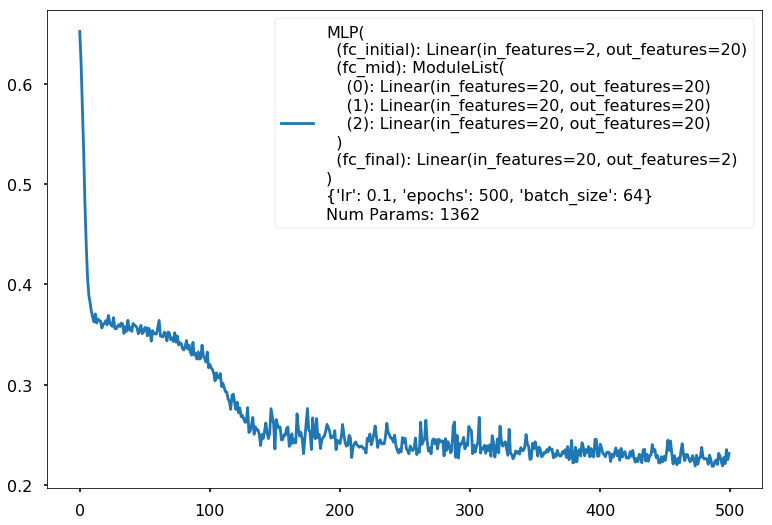
Train acc 0.908333333333
Test acc 0.86875
====================
Additional 3 hidden 100
MLP(
  (fc_initial): Linear(in_features=2, out_features=100)
  (fc_mid): ModuleList(
    (0): Linear(in_features=100, out_features=100)
    (1): Linear(in_features=100, out_features=100)
    (2): Linear(in_features=100, out_features=100)
  )
  (fc_final): Linear(in_features=100, out_features=2)
)
{'lr': 0.1, 'epochs': 1000, 'batch_size': 64}
Num Params: 30802
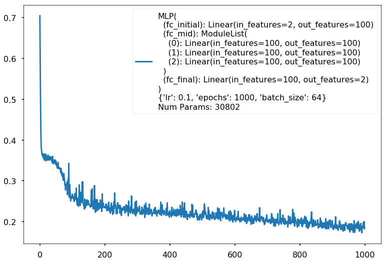
Train acc 0.929166666667
Test acc 0.88125
====================
Additional 3 hidden 1000
MLP(
  (fc_initial): Linear(in_features=2, out_features=1000)
  (fc_mid): ModuleList(
    (0): Linear(in_features=1000, out_features=1000)
    (1): Linear(in_features=1000, out_features=1000)
    (2): Linear(in_features=1000, out_features=1000)
  )
  (fc_final): Linear(in_features=1000, out_features=2)
)
{'lr': 0.1, 'epochs': 1000, 'batch_size': 64}
Num Params: 3008002
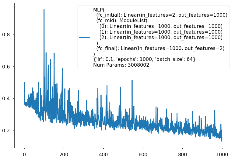
Train acc 0.958333333333
Test acc 0.875